Basic Optical Fiber Metrics

Scott Prahl

Sept 2023

# Jupyterlite support for ofiber
try:
    import micropip
    await micropip.install("ofiber")
except ModuleNotFoundError:
    pass

import matplotlib.pyplot as plt
import numpy as np
import ofiber

%config InlineBackend.figure_format='retina'

The relative refractive index or Δ

Compare result with an approximation.

n_clad= 1.48
n_core = 1.5
Δ_approx = (n_core-n_clad)/n_core
print("Δ = %.5f (approximation)"%Δ_approx)
Δ = ofiber.relative_refractive_index(n_core,n_clad)  #exact
print("Δ = %.5f"%Δ)

Δ = 0.01333 (approximation)
Δ = 0.01324

Numerical Aperture of a step index fiber

A convenience method to find the numerical aperture given the core and cladding index.

n_clad= 1.48
n_core = 1.5
Δ = (n_core-n_clad)/n_core

NA = n_core*np.sqrt(2*Δ)
print("NA    = %.4f (approximation)"%NA)
NA = ofiber.numerical_aperture(n_core,n_clad)
print("NA    = %.4f"%NA)

NA    = 0.2449 (approximation)
NA    = 0.2441

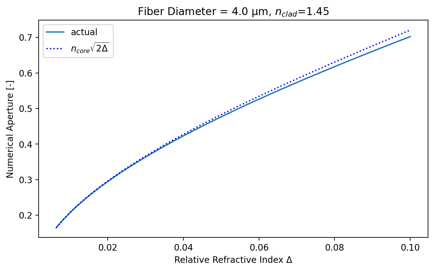
We can easily make plots. Here is the variation of the exact numerical aperture and that obtained with the approximation to \(\Δ\)

r_core=2e-6
n_clad= 1.45  # pure SiO2

Δ = np.linspace(0.0064,0.1,50)
n_core = n_clad/(1-Δ)

NA = ofiber.numerical_aperture(n_core,n_clad)

plt.plot(Δ,NA,label='actual')
plt.plot(Δ,n_core*np.sqrt(2*Δ),':b',label=r'$n_{core}\sqrt{2\Delta}$')
plt.xlabel(r'Relative Refractive Index Δ')
plt.ylabel('Numerical Aperture [-]')
plt.title(r'Fiber Diameter = %.1f µm, $n_{clad}$=%.2f'%(2*r_core*1e6,n_clad))

plt.legend()
plt.show()

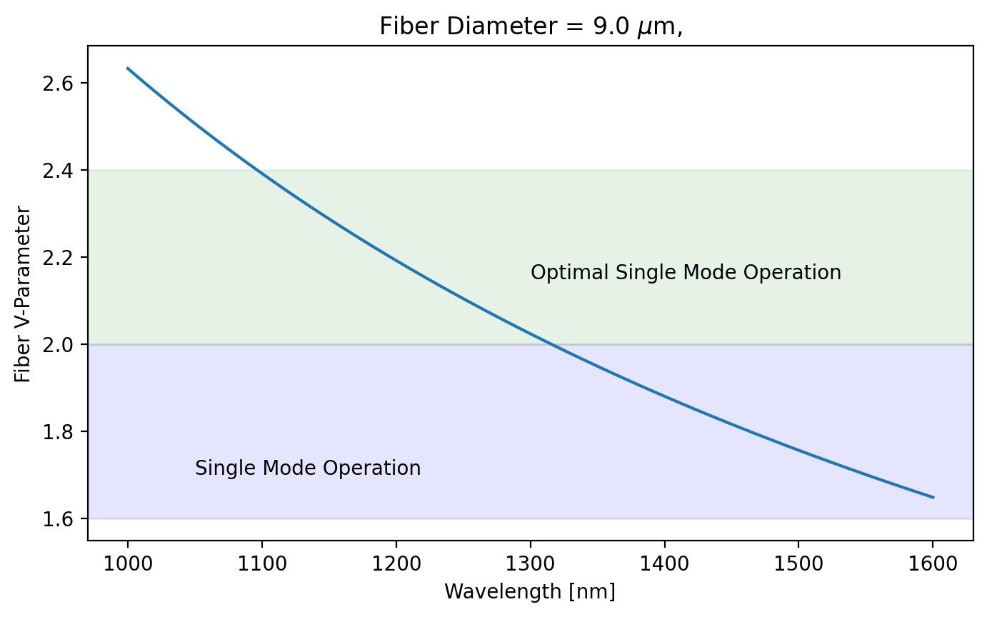
The V-parameter for a fiber

This helps characterize the number of modes in a fiber. If \(V\gg 2.4\) then the number of modes is

\[N \approx \frac{V^2}{2}\]

d=9e-6                                    # m
r_core = d/2
λ = np.linspace(1000,1600,100)*1e-9 # m

clad = ofiber.doped_glass(0)     # pure SiO2
n_clad = ofiber.n(clad,λ)

core = ofiber.doped_glass(0.02)  # 2% GeO2
n_core = ofiber.n(core,λ)

NA = ofiber.numerical_aperture(n_core,n_clad)
V = ofiber.V_parameter(r_core,NA,λ)

plt.plot(λ*1e9,V)
plt.axhspan(1.6,2.0,color='blue',alpha=0.1)
plt.axhspan(2.0,2.4,color='green',alpha=0.1)

plt.ylabel(r'Fiber V-Parameter')
plt.xlabel('Wavelength [nm]')
plt.title(r'Fiber Diameter = %.1f $\mu$m,'%(d*1e6))
plt.text(1300, 2.15, "Optimal Single Mode Operation")
plt.text(1050, 1.7, "Single Mode Operation")

plt.show()

The cutoff wavelength for a fiber

r_core = 2e-6    # m
Δ      = 0.0064
n_clad = 1.45
n_core = n_clad/(1-Δ)
NA     = n_core*np.sqrt(2*Δ)
lambdac=ofiber.cutoff_wavelength(r_core, NA)

print("Cutoff wavelength is %.0f nm"%(lambdac*1e9))

Cutoff wavelength is 863 nm

Example page 21 in Powers

The effect of a graded index fiber on the cutoff wavelength.

d=8e-6      # m
r_core=d/2  # m
λ = 1300e-9 # m

n_core = 1.46
V = 2.1
NA = V/2/np.pi*λ/r_core

lambdac=ofiber.cutoff_wavelength(r_core, NA)
print("Cutoff wavelength is %.0f nm (step-index)"%(lambdac*1e9))

lambdac=ofiber.cutoff_wavelength(r_core, NA, q=2)
print("Cutoff wavelength is %.0f nm (parabolic fiber)"%(lambdac*1e9))

Cutoff wavelength is 1135 nm (step-index)
Cutoff wavelength is 803 nm (parabolic fiber)

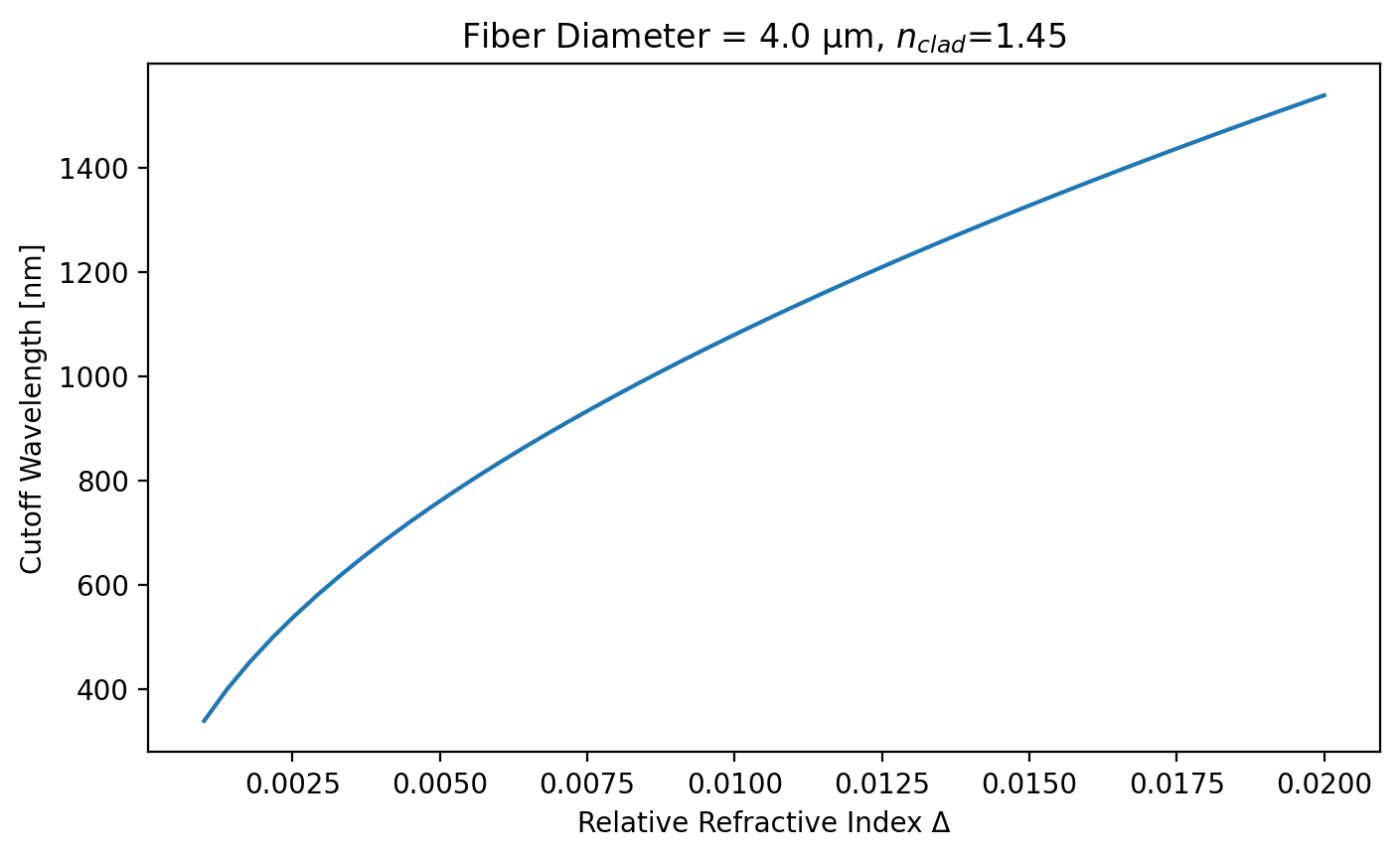
Finally, how does the cutoff wavelength depend on the relative refractive index?

r_core=2e-6
n_clad= 1.45
Δ = np.linspace(0.001,0.02,50)

n_core = n_clad/(1-Δ)
NA = ofiber.numerical_aperture(n_core,n_clad)
lambdac = ofiber.cutoff_wavelength(r_core, NA)

plt.plot(Δ,lambdac*1e9)
plt.xlabel(r'Relative Refractive Index Δ')
plt.ylabel('Cutoff Wavelength [nm]')
plt.title(r'Fiber Diameter = %.1f µm, $n_{clad}$=%.2f'%(2*r_core*1e6, n_clad))
plt.show()