Far-field Irradiance and Numerical Aperture
Matthew Spotnitz
Feb 2024
In this notebook, we follow “Foundations for Guided-Wave Optics” by Chin-Lin Chen (2006) and
reproduce Figures 10.3−10.6
plot the optical fiber emission angle for the fundamental mode for a range of core radii \(a\).
plot the far-field emission
[ ]:
%config InlineBackend.figure_format='retina'

import sys
import scipy
import scipy.optimize
import scipy.signal
import numpy as np
import matplotlib.pyplot as plt

if sys.platform == "emscripten":
    import micropip
    await micropip.install("ofiber")

import ofiber
[ ]:
def dB(x):
    return 10 * np.log10(x)
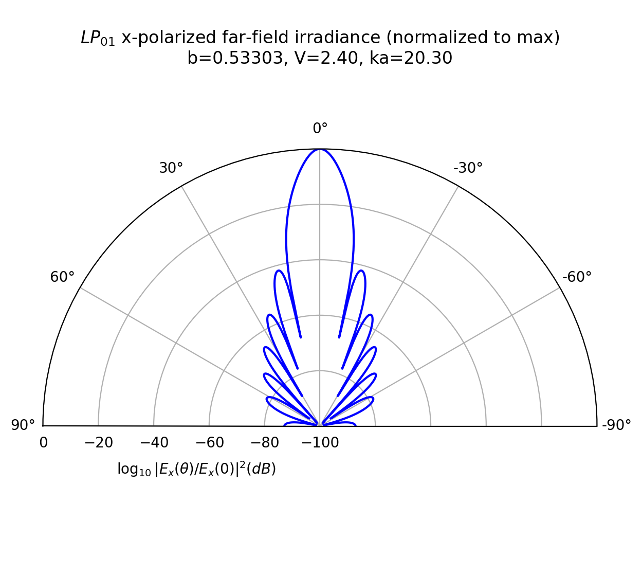
Plotting Far-Field Irradiance
To plot the far-field (Fraunhofer) irradiance, we select an arbitrary point in the far-field, say \(r=100\lambda\). The irradiance at this distance from the fiber face will depend on both the polar angle \(\theta\) and the azimuthal angle \(\phi\). Since the azimuthal distribution is just \(\cos^2 \ell\phi\), it is relatively uninteresting. To simplify the plot, we integrate the irradiance over all azimuthal angles and normalize by the maximum at \(\theta=0°\).
[27]:
k = 1
ell = 0  # azimuthal mode ℓ
a = 20.3  # k=1 so ka=20.3
V = 2.4
b = 0.53303  # this value corresponds to the LP_01 mode
lambda0 = 2 * np.pi  # so that k=1 and ka=a=20.3
r = 100 * lambda0  # 100 wavelengths from the fiber face

theta = np.radians(np.linspace(-90, 90, 501))

# calculate the normalized irradiance
IFF = ofiber.FF_polar_irradiance_x(r, theta, ell, lambda0, a, V, b)
F = IFF / np.max(IFF)
Now plot the irradiance to reproduce Chen figure 10.3
[28]:
title = "$LP_{01}$ x-polarized far-field irradiance (normalized to max)\n"
title += r"b=%.5f, V=%.2f, ka=%.2f" % (b, V, a)
rlabel = r"$\log_{10}|E_x(\theta)/E_x(0)|^2 (dB)$"

fig, ax = plt.subplots(subplot_kw={"projection": "polar"}, figsize=(7, 7))
ax.plot(theta, dB(F), "b")
ax.set_theta_zero_location("N")
ax.set_thetalim(np.pi / 2, -np.pi / 2)
ax.set_ylim(-100, 0)
ax.grid(True)
ax.set_title(title, va="bottom", pad=-40)
plt.figtext(0.23, 0.23, rlabel, ha="left", va="bottom")
plt.show()
Emission angle variation with the radius of the fiber core.
We seek the the fundamental mode emission angle for the \(\text{LP}_{01}\) cylindrical fiber mode over a range of core radii.
Calculate the normalized propagation constant vs core radii
Calculate the relative refractive index \(\Delta\), numerical aperture NA, and generalized frequency \(V\) assuming fixed \(n_{\mathrm{core}}\) and \(n_{\mathrm{cladding}}\) refractive indices.
Here we find the \(b\) values using the imporoved LP_mode_value from version 0.8.0 of ofiber.
[29]:
ell = 0
em = 1
n_core = 1.589
n_cladding = 1.48
lambda0 = 0.550  # center wavelength over visible spectrum 0.400-0.700 µm
a = np.linspace(2, 15, num=131)  # core radii from 2-15 microns

Delta = ofiber.relative_refractive_index(n_core, n_cladding)
NA = ofiber.numerical_aperture_from_Delta(n_core, Delta)
V = ofiber.V_parameter(a, NA, lambda0)
b_ofiber = ofiber.LP_mode_value(V, ell, em)
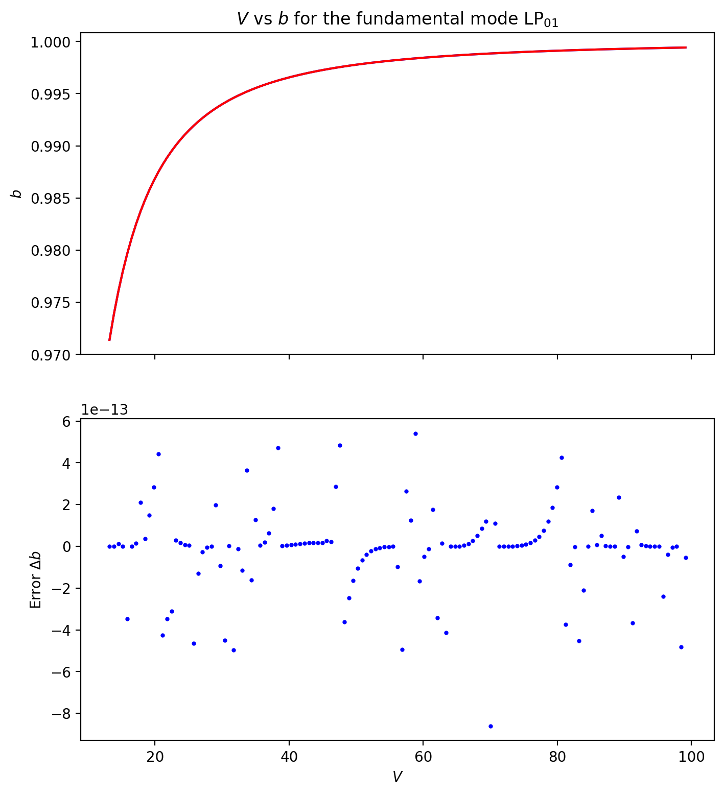
Alternate method
The routine ofiber.LP_mode_value (version 0.7.1 of ofiber and earlier) breaks down for very large \(V\) values, so an alternate method, taking advantage of the monotonic increase of \(b(V)\), is used.
The routine ofiber.LP_mode_value works for the first \(V\) value. We use this to find the lower bound for all remaining \(b\) values. (Using a lower bound of \(b=0\) in the bracketing algorithm may lead to errors.)
[30]:
ell = 0
em = 1
n_core = 1.589
n_cladding = 1.48
lambda0 = 0.550  # center wavelength over visible spectrum 0.400-0.700 µm
a = np.linspace(2, 15, num=131)  # core radii from 2-15 microns

Delta = ofiber.relative_refractive_index(n_core, n_cladding)
NA = ofiber.numerical_aperture_from_Delta(n_core, Delta)
V = ofiber.V_parameter(a, NA, lambda0)

b = np.zeros_like(V)
b[0] = ofiber.LP_mode_value(V[0], ell, em)

for i in range(1, len(V)):
    b[i] = (
        scipy.optimize.root_scalar(f=ofiber.cylinder_step._cyl_mode_eqn, args=(V[i], 0), bracket=(b[i - 1], 1))
    ).root
[50]:
# plot both versions.  they yield equal values
plt.figure(figsize=(8, 9))
plt.subplot(2, 1, 1)
# plt.xlabel(r'$V$')
plt.gca().set_xticklabels([])
plt.ylabel(r"$b$")
plt.plot(V, b, color="blue")
plt.plot(V, b_ofiber, color="red")
plt.title(r"$V$ vs $b$ for the fundamental mode $\text{LP}_{01}$")
# plt.show()

# plt.figure(figsize=(8,4.5))
plt.subplot(2, 1, 2)
plt.xlabel(r"$V$")
plt.ylabel(r"Error $\Delta b$")
plt.plot(V, b - b_ofiber, "o", markersize=2, color="blue")
# plt.title("Difference in calculation of $b$")
plt.show()
Calculate the irradiance for each core radius at all polar angles 0-90°
Calculate the irradiance as a function of polar angle for every fiber core radius. We first create a matrix of size \(N_{\theta} \times N_{a}\) and then fill each column with the far-field irradiance at each polar angle.
[38]:
theta = np.radians(np.linspace(0, 90, 1801))
I_a_theta = np.zeros((len(theta), len(a)))

r = 100
ell = 0
lambda0 = 0.55
for i in range(len(V)):
    I_a_theta[:, i] = ofiber.FF_polar_irradiance_x(r, theta, ell, lambda0, a[i], V[i], b[i])
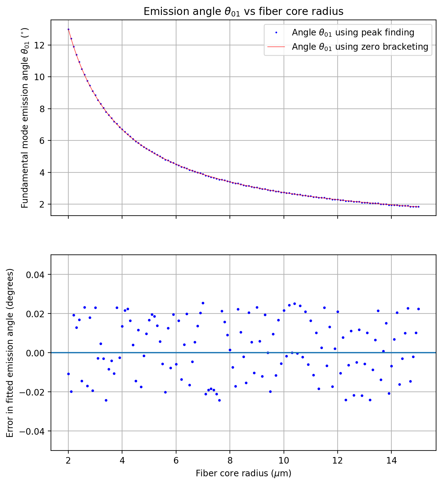
Extract the polar angle of the minimum of the central irradiance lobe for each \(a\) value.
Find the first minimum \(\Theta_{01}\) of \(I \propto |E_{\mathrm{FF}x}|^{2}\) when starting the search from \(\Theta = 0\) and increasing. (For the fundamental mode, the first minimum is always at a nonzero \(\Theta\).)
We demonstrate here two methods, in this order: searching the intensity for its first minimum, and directly solving for the first zero of the polar factor in the field pattern.
[39]:
firstMin = np.zeros_like(a)

for i in range(a.size):
    peaks, _ = scipy.signal.find_peaks(-I_a_theta[:, i])
    firstMin[i] = theta[peaks[0]]
[40]:
FF_node = ofiber.FF_node_polar_angle(V, ell, em)
Convert \(\theta_{01}\) from radians to degrees, to ease visualization.
[41]:
k = 2 * np.pi / lambda0 # free-space wavenumber
[42]:
firstMinDeg = np.degrees(firstMin) # convert the first min angle peak to degrees
[43]:
FF_node_deg = np.degrees(np.arcsin(FF_node / (k * a))) # convert k*a*sin Θ to Θ in degrees
Plot of the two methods, and their difference:
[60]:
plt.figure(figsize=(8, 9))
plt.subplot(2, 1, 1)
# plt.xlabel(r'Fiber core radius $a$ ($\mu$m)')
plt.gca().set_xticklabels([])
plt.ylabel(r"Fundamental mode emission angle $\theta_{01}$ ($^{\circ}$)")
plt.title(r"Emission angle $\theta_{01}$ vs fiber core radius")
plt.plot(a, firstMinDeg, "ob", label=r"Angle $\theta_{01}$ using peak finding", markersize=1)
plt.plot(a, FF_node_deg, label=r"Angle $\theta_{01}$ using zero bracketing", lw=0.5, color="red")
plt.grid()
plt.legend()
# plt.show()

# plt.figure(figsize=(8,4.5))
plt.subplot(2, 1, 2)
plt.xlabel(r"Fiber core radius ($\mu$m)")
plt.ylabel("Error in fitted emission angle (degrees)")
# plt.title(r'Emission angle $\theta_{01}$ vs core radius $a$')
plt.plot(a, firstMinDeg - FF_node_deg, "ob", lw=0.5, markersize=2)
plt.axhline(0)
plt.ylim(-0.05, 0.05)
plt.grid(True)
plt.show()
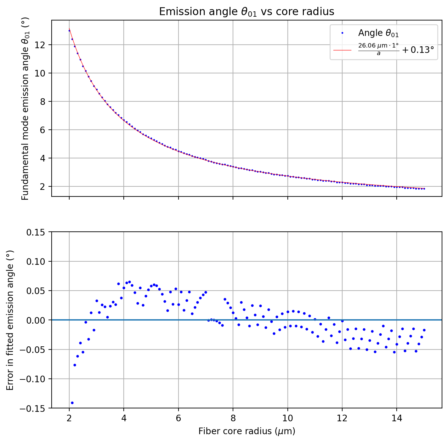
Plot of emission angle vs fiber radius
Define the fit function for the angle \(\theta_{01}\) vs \(a\) curve.
[53]:
def fxinv(radius, b, c):
    return b / radius + c
Fit the \(x^{-1}\) function fxinv to the firstMinDeg as a function of the fiber radius. First convert \(\theta_{01}\) from radians to degrees, to ease visualization.
[54]:
firstMinDeg = np.degrees(firstMin)  # convert the first min angle peak to degrees
popt, pcov = scipy.optimize.curve_fit(fxinv, a, firstMinDeg)
fit = fxinv(a, popt[0], popt[1])
Plot the emission angle calculations and the fit function. We see that in this regime, \(\theta_{01}(a) = \frac{b}{a} + c\). The inverse of this fit is \(\frac{b}{\theta - c} = a\).
[61]:
plt.figure(figsize=(8, 8))
plt.subplot(2, 1, 1)
# plt.xlabel(r'Fiber core radius ($\mu$m)')
plt.gca().set_xticklabels([])
plt.ylabel(r"Fundamental mode emission angle $\theta_{01}$ (°)")
plt.title(r"Emission angle $\theta_{01}$ vs core radius")
plt.plot(a, firstMinDeg, "ob", label=r"Angle $\theta_{01}$", markersize=1)
s = r"$\frac{%5.2f \ \mu \text{m}\cdot 1°}{a} + %5.2f°$" % tuple(popt)
plt.plot(a, fit, label=s, lw=0.5, color="red")
plt.grid()
plt.legend()

plt.subplot(2, 1, 2)
plt.xlabel(r"Fiber core radius ($\mu$m)")
plt.ylabel("Error in fitted emission angle (°)")
# plt.title(r'Emission angle $\theta_{01}$ vs core radius')
plt.plot(a, firstMinDeg - fit, "ob", lw=0.5, markersize=2)
plt.axhline(0)
plt.ylim(-0.15, 0.15)
plt.grid(True)
plt.show()
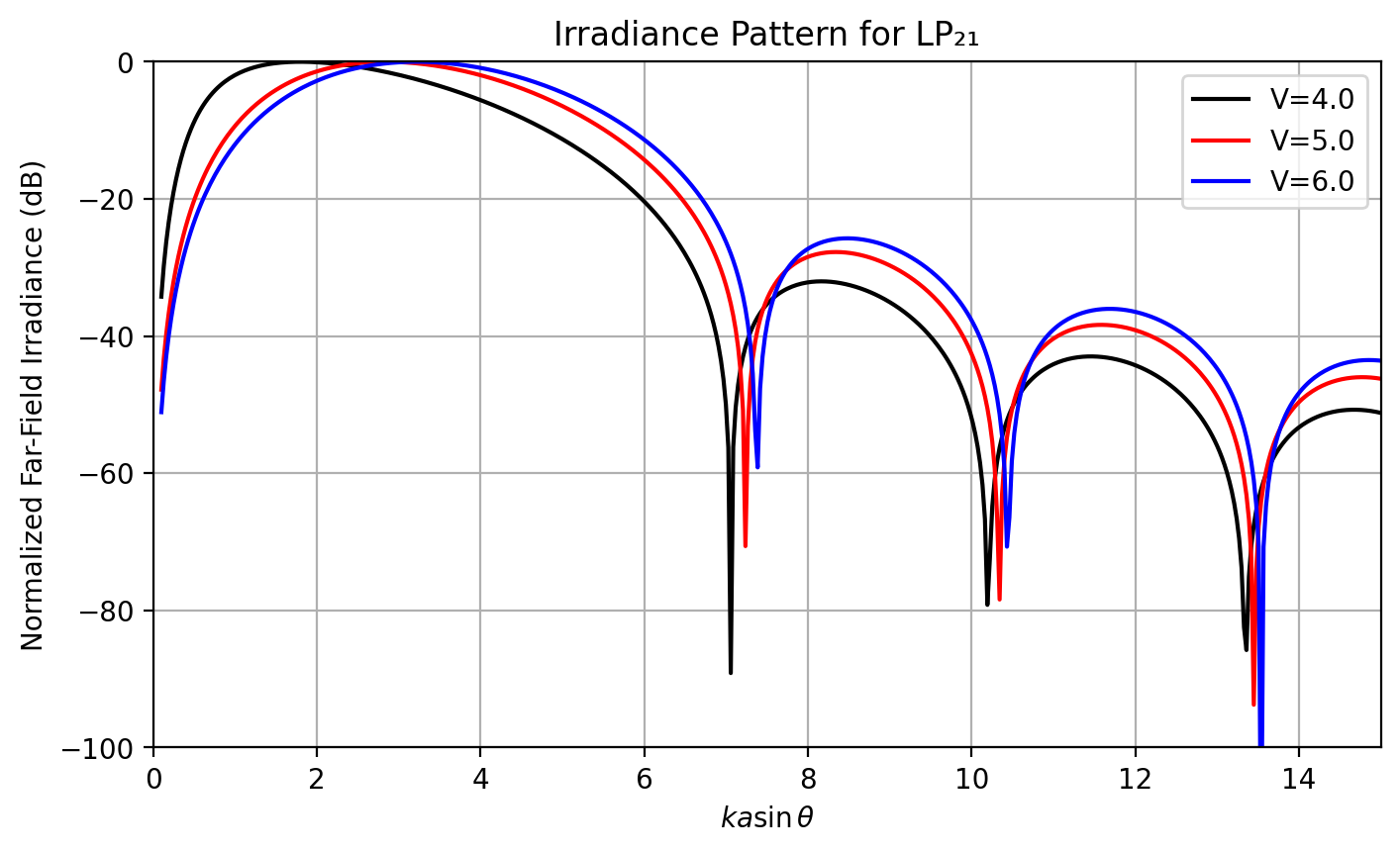
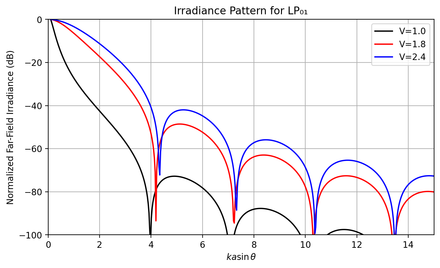
Variation with ka sin𝜃
Reproducing figures 10.4, 10.5, and 10.6 from Chen.
[17]:
# Figure 10.4, page 264 in Chen
kasin = np.linspace(0.1, 15, 500)

ell = 0
em = 1
lambda0 = 1  # microns
r = 100 * lambda0  # microns
a = 3  # microns

k = 2 * np.pi / lambda0
theta = np.arcsin(kasin / (k * a))

plt.figure(figsize=(8, 4.5))
plt.title("Irradiance Pattern for LP₀₁")
V = 1
b = ofiber.LP_mode_value(V, ell, em)
ff = ofiber.FF_polar_irradiance_x(r, theta, ell, lambda0, a, V, b)
ff /= max(ff)
plt.plot(kasin, dB(ff), color="black", label="V=%.1f" % V)

V = 1.8
b = ofiber.LP_mode_value(V, ell, em)
ff = ofiber.FF_polar_irradiance_x(r, theta, ell, lambda0, a, V, b)
ff /= max(ff)
plt.plot(kasin, dB(ff), color="red", label="V=%.1f" % V)

V = 2.4
b = ofiber.LP_mode_value(V, ell, em)
ff = ofiber.FF_polar_irradiance_x(r, theta, ell, lambda0, a, V, b)
ff /= max(ff)
plt.plot(kasin, dB(ff), color="blue", label="V=%.1f" % V)

plt.legend()
plt.ylim(-100, 0)
plt.xlim(0, 15)
plt.grid(True)
plt.xlabel(r"$k a \sin\theta$")
plt.ylabel("Normalized Far-Field Irradiance (dB)")
plt.show()
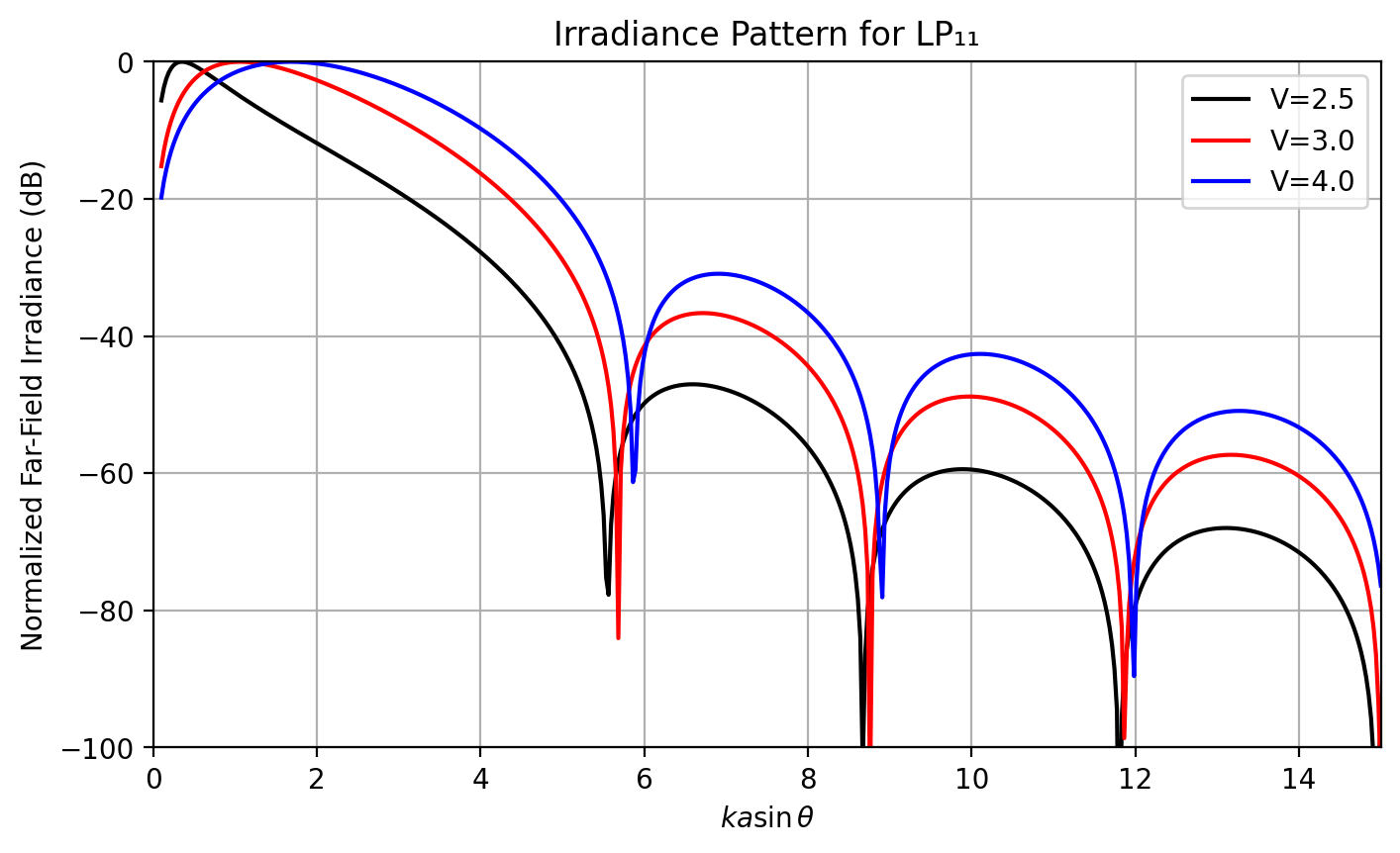
[18]:
# Figure 10.5, page 264 in Chen
kasin = np.linspace(0.1, 15, 500)

ell = 1
em = 1
lambda0 = 1  # microns
r = 100 * lambda0  # microns
a = 3  # microns

k = 2 * np.pi / lambda0
theta = np.arcsin(kasin / (k * a))

plt.figure(figsize=(8, 4.5))
plt.title("Irradiance Pattern for LP₁₁")
V = 2.5
b = ofiber.LP_mode_value(V, ell, em)
ff = ofiber.FF_polar_irradiance_x(r, theta, ell, lambda0, a, V, b)
ff /= max(ff)
plt.plot(kasin, dB(ff), color="black", label="V=%.1f" % V)

V = 3.0
b = ofiber.LP_mode_value(V, ell, em)
ff = ofiber.FF_polar_irradiance_x(r, theta, ell, lambda0, a, V, b)
ff /= max(ff)
plt.plot(kasin, dB(ff), color="red", label="V=%.1f" % V)

V = 4.0
b = ofiber.LP_mode_value(V, ell, em)
ff = ofiber.FF_polar_irradiance_x(r, theta, ell, lambda0, a, V, b)
ff /= max(ff)
plt.plot(kasin, dB(ff), color="blue", label="V=%.1f" % V)

plt.legend()
plt.ylim(-100, 0)
plt.xlim(0, 15)
plt.grid(True)
plt.xlabel(r"$k a \sin\theta$")
plt.ylabel("Normalized Far-Field Irradiance (dB)")
plt.show()
[19]:
# Figure 10.6, page 265 in Chen
kasin = np.linspace(0.1, 15, 500)

ell = 2
em = 1
lambda0 = 1  # microns
r = 100 * lambda0  # microns
a = 3  # microns

k = 2 * np.pi / lambda0
theta = np.arcsin(kasin / (k * a))

plt.figure(figsize=(8, 4.5))
plt.title("Irradiance Pattern for LP₂₁")
V = 4.0
b = ofiber.LP_mode_value(V, ell, em)
ff = ofiber.FF_polar_irradiance_x(r, theta, ell, lambda0, a, V, b)
ff /= max(ff)
plt.plot(kasin, dB(ff), color="black", label="V=%.1f" % V)

V = 5.0
b = ofiber.LP_mode_value(V, ell, em)
ff = ofiber.FF_polar_irradiance_x(r, theta, ell, lambda0, a, V, b)
ff /= max(ff)
plt.plot(kasin, dB(ff), color="red", label="V=%.1f" % V)

V = 6.0
b = ofiber.LP_mode_value(V, ell, em)
ff = ofiber.FF_polar_irradiance_x(r, theta, ell, lambda0, a, V, b)
ff /= max(ff)
plt.plot(kasin, dB(ff), color="blue", label="V=%.1f" % V)

plt.legend()
plt.ylim(-100, 0)
plt.xlim(0, 15)
plt.grid(True)
plt.xlabel(r"$k a \sin\theta$")
plt.ylabel("Normalized Far-Field Irradiance (dB)")
plt.show()