Cylindrical Fibers with step index profile
Scott Prahl
Sept 2023
Graphs and tables from Chapter 8 of Ghatak.
[1]:
%config InlineBackend.figure_format='retina'

import sys
import scipy
import numpy as np
import matplotlib.pyplot as plt
from scipy.optimize import curve_fit

if sys.platform == "emscripten":
    import micropip
    await micropip.install("ofiber")

import ofiber
Single mode in a circular step fiber V=2
(Ghatak Fig 8.1)
Use ofiber.plot_LP_modes to make a quick plot showing the allowed modes.
[2]:
V = 6.5
ell = 0
plt.subplots(1, 2, figsize=(10, 4))
plt.subplot(1, 2, 1)
aplt = ofiber.plot_LP_modes(V, ell)
plt.subplot(1, 2, 2)
ell = 1

aplt = ofiber.plot_LP_modes(V, ell)
aplt.show()

for ell in range(2):
    all_b = ofiber.LP_mode_values(V, ell)
    for i, b in enumerate(all_b):
        print("LP_%d%d, b=%.4f" % (ell, i + 1, b))
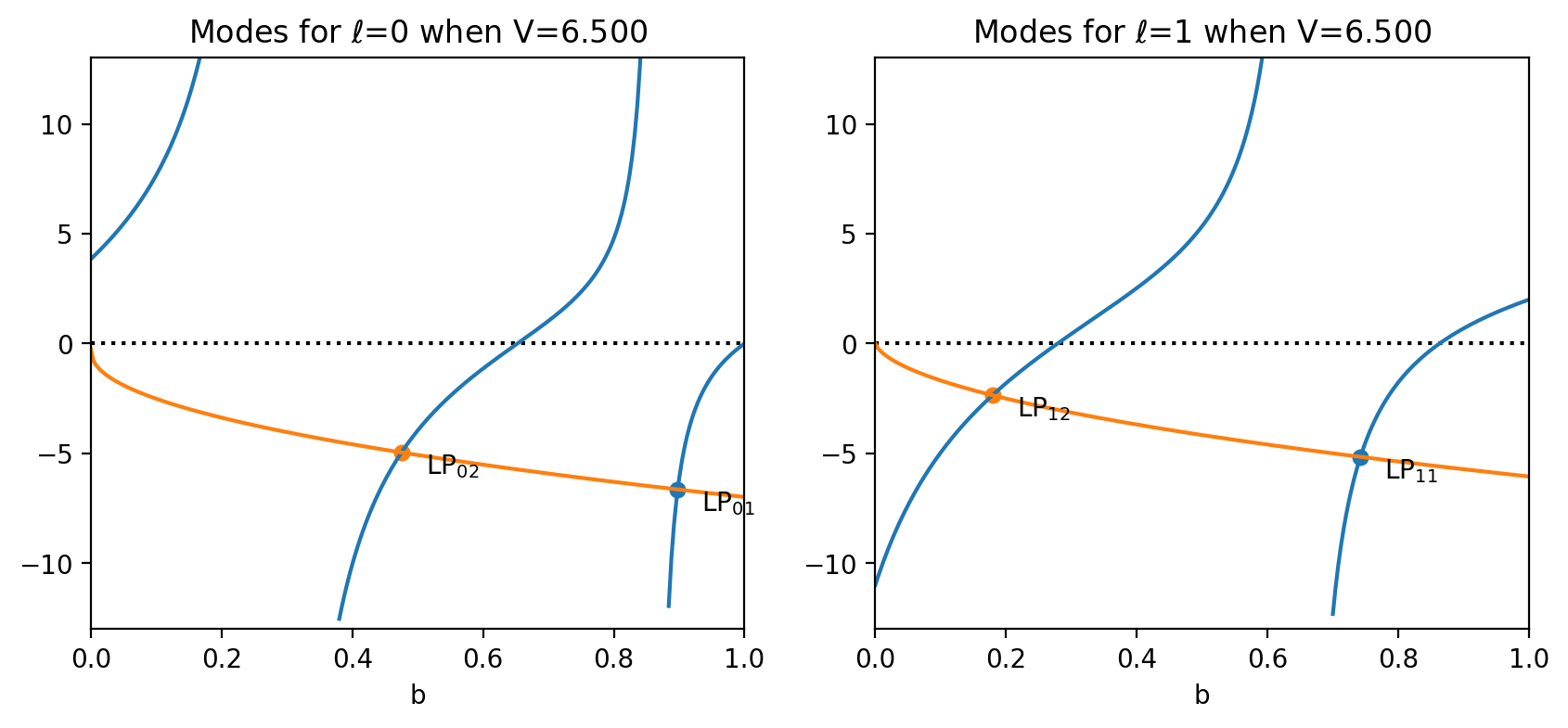
LP_01, b=0.8977
LP_02, b=0.4752
LP_11, b=0.7422
LP_12, b=0.1792
Multiple modes in a circular step fiber V=12.5
Use ofiber.plot_LP_modes to make a quick plot showing the allowed modes.
[3]:
V = 12.5
ell = 0
plt.figure(figsize=(8, 4.5))
aplt = ofiber.plot_LP_modes(V, ell)
aplt.show()

for ell in range(6):
    all_b = ofiber.LP_mode_values(V, ell)
    for i, b in enumerate(all_b):
        print("LP_%d%d, b=%.4f" % (ell, i + 1, b))
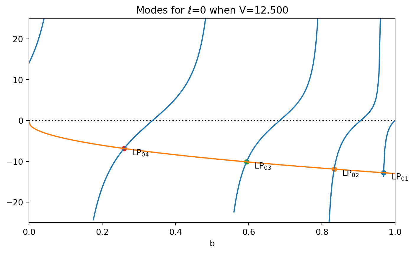
LP_01, b=0.9683
LP_02, b=0.8336
LP_03, b=0.5942
LP_04, b=0.2597
LP_11, b=0.9196
LP_12, b=0.7319
LP_13, b=0.4427
LP_14, b=0.0735
LP_21, b=0.8558
LP_22, b=0.6155
LP_23, b=0.2791
LP_31, b=0.7777
LP_32, b=0.4850
LP_33, b=0.1070
LP_41, b=0.6860
LP_42, b=0.3415
LP_51, b=0.5812
LP_52, b=0.1863
Ghatak Table 8.1
Summarizing all the important parameters for low V-parameter fibers.
[4]:
V = np.linspace(1.5, 2.5, 41)
ell = 0
em = 1
print("  V       b       U       W  wp/r_core MFD/r_core")
for v in V:
    b = ofiber.LP_mode_value(v, ell, em)
    W = v * np.sqrt(b)
    U = v * np.sqrt(1 - b)
    w_p = ofiber.PetermannW(v)
    w_mfd = ofiber.MFD(v)
    print("%.3f %.5f %.5f %.5f %.5f %.5f" % (v, b, U, W, w_p, w_mfd))
  V       b       U       W  wp/r_core MFD/r_core
1.500 0.22925 1.31689 0.71820 1.69342 3.56805
1.525 0.23955 1.32985 0.74640 1.65638 3.47716
1.550 0.24980 1.34252 0.77469 1.62172 3.39317
1.575 0.25997 1.35489 0.80305 1.58923 3.31537
1.600 0.27006 1.36698 0.83148 1.55872 3.24312
1.625 0.28007 1.37880 0.85997 1.53001 3.17585
1.650 0.28997 1.39034 0.88851 1.50295 3.11309
1.675 0.29977 1.40163 0.91709 1.47741 3.05439
1.700 0.30947 1.41267 0.94571 1.45326 2.99939
1.725 0.31905 1.42347 0.97435 1.43040 2.94774
1.750 0.32851 1.43403 1.00303 1.40872 2.89915
1.775 0.33785 1.44436 1.03172 1.38814 2.85335
1.800 0.34707 1.45448 1.06043 1.36858 2.81010
1.825 0.35616 1.46437 1.08914 1.34996 2.76920
1.850 0.36512 1.47406 1.11787 1.33223 2.73045
1.875 0.37396 1.48355 1.14660 1.31531 2.69369
1.900 0.38266 1.49285 1.17533 1.29915 2.65876
1.925 0.39123 1.50195 1.20406 1.28371 2.62552
1.950 0.39967 1.51087 1.23279 1.26893 2.59385
1.975 0.40798 1.51962 1.26150 1.25478 2.56363
2.000 0.41616 1.52818 1.29021 1.24122 2.53477
2.025 0.42421 1.53658 1.31891 1.22820 2.50718
2.050 0.43213 1.54482 1.34760 1.21571 2.48076
2.075 0.43992 1.55290 1.37627 1.20370 2.45544
2.100 0.44758 1.56082 1.40493 1.19216 2.43115
2.125 0.45512 1.56860 1.43357 1.18105 2.40783
2.150 0.46252 1.57622 1.46220 1.17035 2.38541
2.175 0.46981 1.58371 1.49080 1.16003 2.36385
2.200 0.47697 1.59106 1.51938 1.15009 2.34308
2.225 0.48401 1.59827 1.54795 1.14049 2.32308
2.250 0.49093 1.60536 1.57649 1.13122 2.30379
2.275 0.49773 1.61231 1.60501 1.12227 2.28517
2.300 0.50442 1.61915 1.63351 1.11361 2.26719
2.325 0.51099 1.62586 1.66199 1.10523 2.24981
2.350 0.51744 1.63246 1.69044 1.09713 2.23301
2.375 0.52379 1.63894 1.71887 1.08928 2.21675
2.400 0.53003 1.64531 1.74727 1.08168 2.20101
2.425 0.53616 1.65157 1.77565 1.07431 2.18576
2.450 0.54218 1.65773 1.80400 1.06716 2.17098
2.475 0.54810 1.66379 1.83233 1.06022 2.15665
2.500 0.55392 1.66974 1.86064 1.05349 2.14274
Example 8.1 Figure 8.2
[5]:
n_clad = 1.45
Delta = 0.0064
r_core = 3.0  # microns
λ = 1.546  # microns

n_core = n_clad / np.sqrt(1 - 2 * Delta)
NA = np.sqrt(n_core**2 - n_clad**2)
V = r_core * (2 * np.pi / λ) * NA

plt.subplots(1, 2, figsize=(10, 4), sharey=True)
plt.subplot(1, 2, 1)
plt.plot([0, r_core, r_core, 2 * r_core], [n_core, n_core, n_clad, n_clad], color="blue")
for ell in range(6):
    all_b = ofiber.LP_mode_values(V, ell)
    for b in all_b:
        bt = np.sqrt(n_clad**2 + all_b * (n_core**2 - n_clad**2))
        plt.plot([0, r_core], [bt, bt], "--r")

plt.ylim(1.445, 1.46)
plt.title("V=%.1f, λ=%.4f microns" % (V, λ))
plt.xlabel("radius (microns)")
plt.ylabel("Refractive Index")


λ = 0.4757  # microns
n_core = n_clad / np.sqrt(1 - 2 * Delta)
NA = np.sqrt(n_core**2 - n_clad**2)
V = r_core * (2 * np.pi / λ) * NA

plt.subplot(1, 2, 2)

plt.plot([0, r_core, r_core, 2 * r_core], [n_core, n_core, n_clad, n_clad], color="blue")
for ell in range(6):
    all_b = ofiber.LP_mode_values(V, ell)
    for b in all_b:
        bt = np.sqrt(n_clad**2 + all_b * (n_core**2 - n_clad**2))
        plt.plot([0, r_core], [bt, bt], "--r")

plt.ylim(1.445, 1.46)
plt.title("V=%.1f, λ=%.4f microns" % (V, λ))
plt.xlabel("radius (microns)")
# plt.ylabel("Refractive Index")

plt.show()
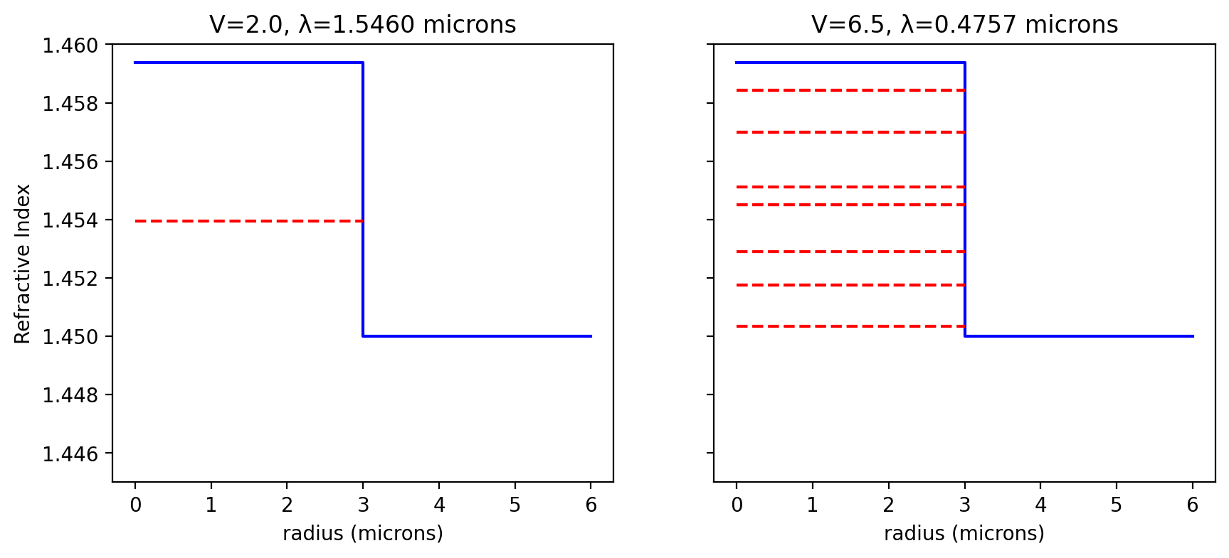
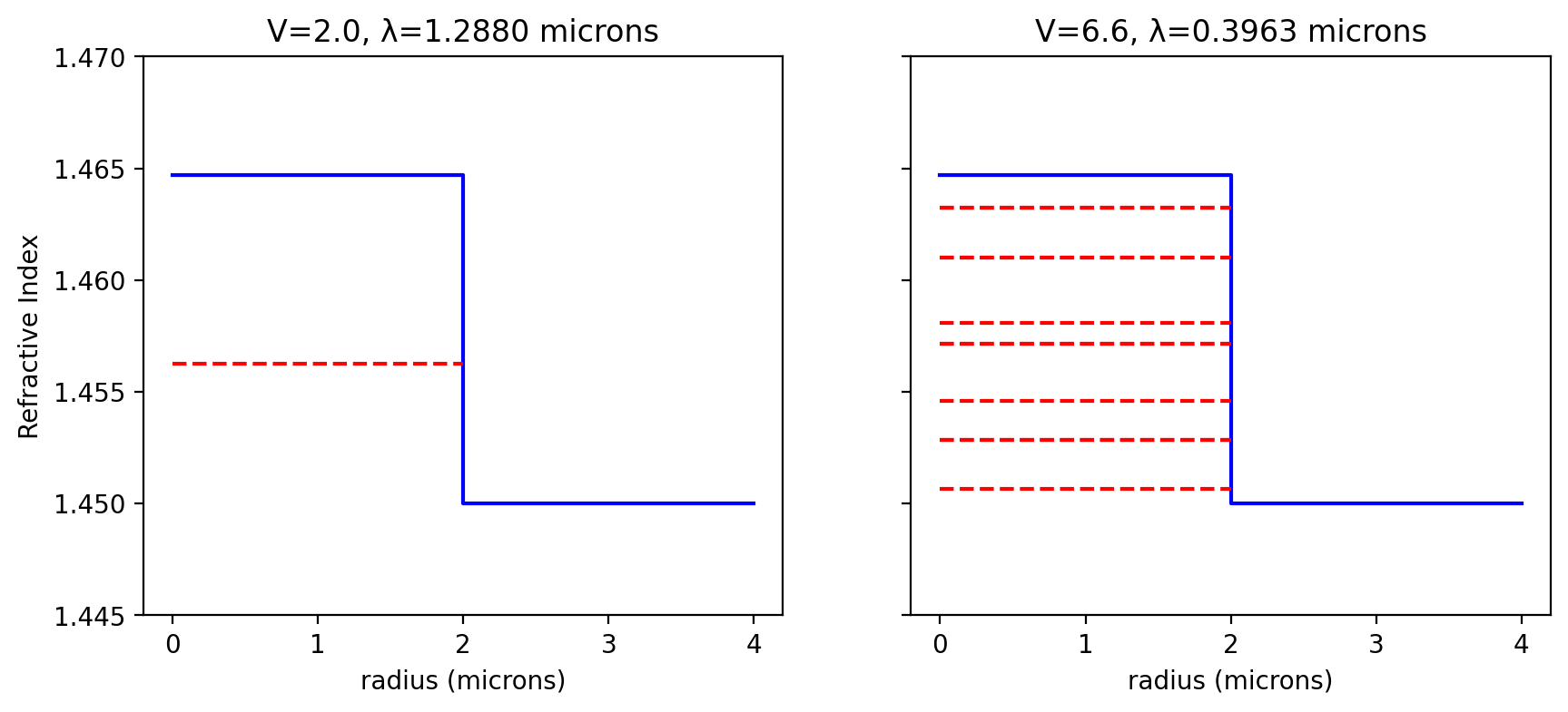
Figure 8.3
[6]:
n_clad = 1.45
Delta = 0.010
r_core = 2.0  # microns

λ = 1.288  # microns
n_core = n_clad / np.sqrt(1 - 2 * Delta)
NA = np.sqrt(n_core**2 - n_clad**2)
V = r_core * (2 * np.pi / λ) * NA

plt.subplots(1, 2, figsize=(10, 4), sharey=True)
plt.subplot(1, 2, 1)
plt.plot([0, r_core, r_core, 2 * r_core], [n_core, n_core, n_clad, n_clad], color="blue")
for ell in range(6):
    all_b = ofiber.LP_mode_values(V, ell)
    for b in all_b:
        bt = np.sqrt(n_clad**2 + all_b * (n_core**2 - n_clad**2))
        plt.plot([0, r_core], [bt, bt], "--r")
plt.ylim(1.445, 1.47)
plt.title("V=%.1f, λ=%.4f microns" % (V, λ))
plt.xlabel("radius (microns)")
plt.ylabel("Refractive Index")


λ = 0.3963  # microns
n_core = n_clad / np.sqrt(1 - 2 * Delta)
NA = np.sqrt(n_core**2 - n_clad**2)
V = r_core * (2 * np.pi / λ) * NA

plt.subplot(1, 2, 2)
plt.plot([0, r_core, r_core, 2 * r_core], [n_core, n_core, n_clad, n_clad], color="blue")
for ell in range(6):
    all_b = ofiber.LP_mode_values(V, ell)
    for b in all_b:
        bt = np.sqrt(n_clad**2 + all_b * (n_core**2 - n_clad**2))
        plt.plot([0, r_core], [bt, bt], "--r")

plt.ylim(1.445, 1.47)
plt.title("V=%.1f, λ=%.4f microns" % (V, λ))
plt.xlabel("radius (microns)")
# plt.ylabel("Refractive Index")

plt.show()
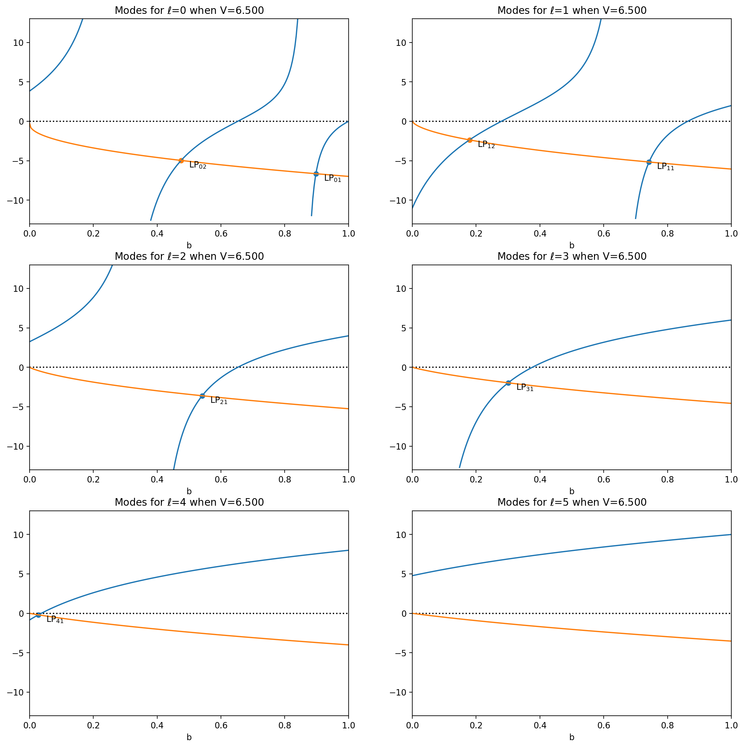
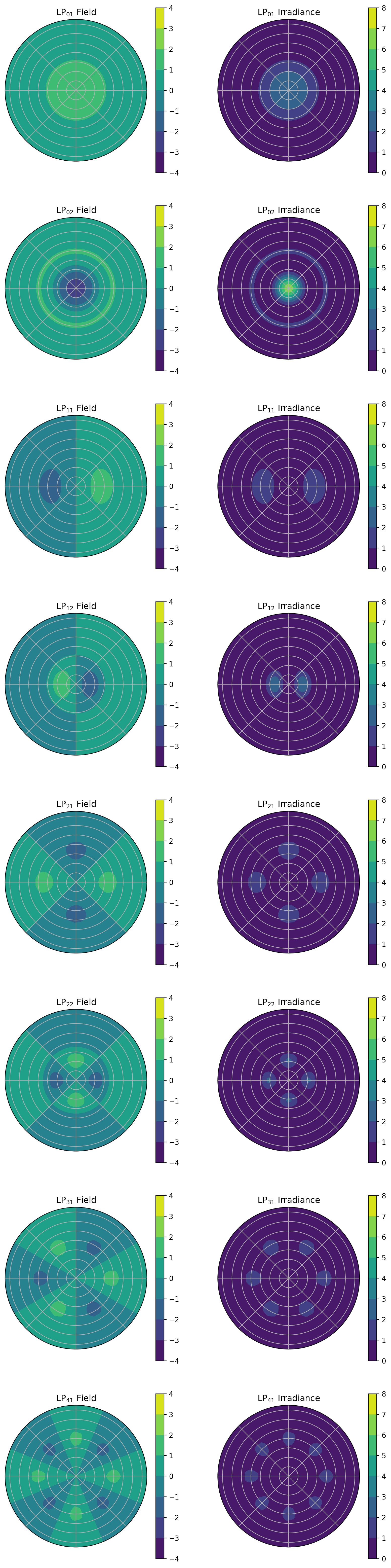
Ghatak Figure 8.4
[7]:
V = 6.5

plt.subplots(3, 2, figsize=(15, 15), squeeze=True)
for ell in range(6):
    aplt.subplot(3, 2, ell + 1)
    aplt = ofiber.plot_LP_modes(V, ell)

aplt.show()
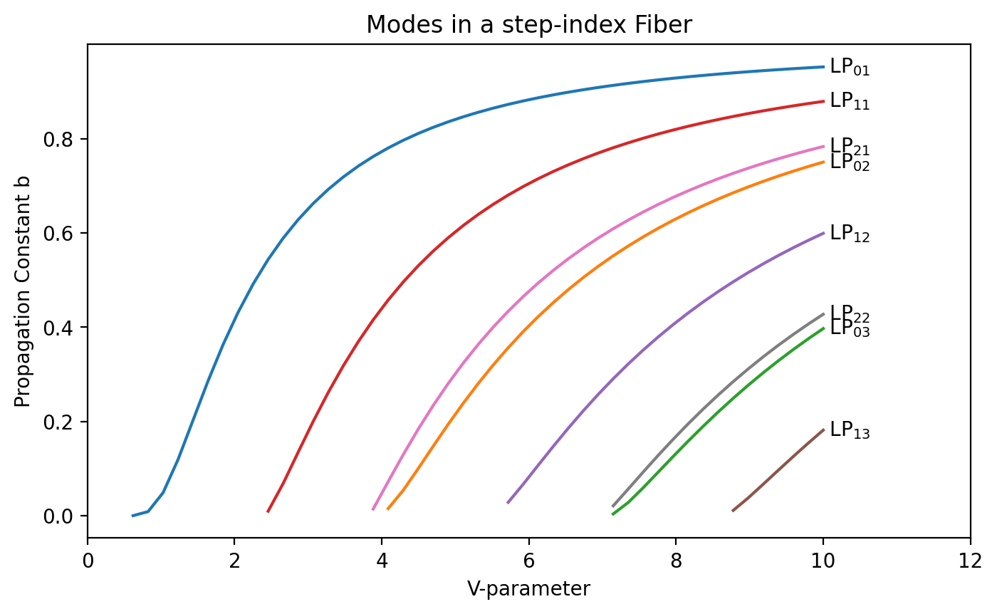
Variation of normalized propagation constant with V
Ghatak Figure 8.5
[8]:
V = np.linspace(0.01, 10, 50)
b = np.empty_like(V)

plt.figure(figsize=(8, 4.5))
for ell in range(3):
    for em in range(1, 4):
        for i in range(len(V)):
            b[i] = ofiber.LP_mode_value(V[i], ell, em)
        plt.plot(V, b)
        plt.annotate(r" LP$_{%d%d}$" % (ell, em), xy=(10, b[-1]), va="center")

plt.xlim(0, 12)
plt.xlabel("V-parameter")
plt.ylabel("Propagation Constant b")
plt.title("Modes in a step-index Fiber")
plt.show()
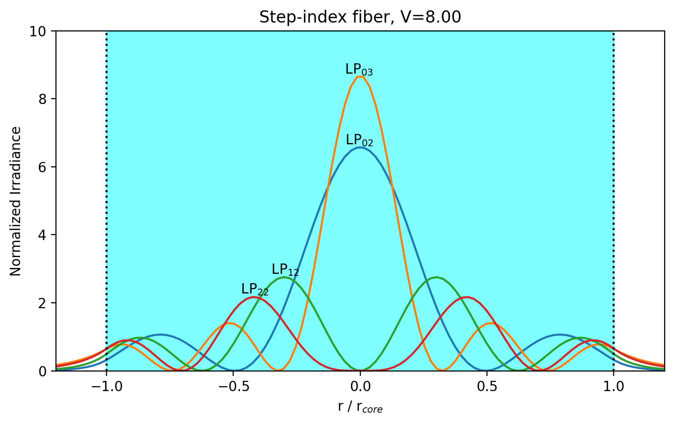
Radial Intensity distributions
Ghatak Figure 8.6
[30]:
plt.subplots(figsize=(8, 4.5))
r_over_a = np.linspace(-1.2, 1.2, 100)
V = 8
for ell in range(3):
    for em in range(2, 4):
        b = ofiber.LP_mode_value(V, ell, em)
        if b is None:
            continue
        irradiance = ofiber.LP_radial_irradiance(V, b, ell, r_over_a)
        i = np.argmax(irradiance)

        plt.plot(r_over_a, irradiance)
        plt.annotate(r" LP$_{%d%d}$" % (ell, em), xy=(r_over_a[i], irradiance[i]), va="bottom", ha="center")

plt.xlabel("r / r$_{core}$")
plt.ylabel("Normalized Irradiance")
plt.plot([-1, -1], [0, 10], ":k")
plt.plot([1, 1], [0, 10], ":k")
plt.axvspan(-1, 1, color="cyan", alpha=0.5)
plt.title("Step-index fiber, V=%.2f" % V)
plt.ylim(0, 10)
plt.xlim(-1.2, 1.2)
plt.show()
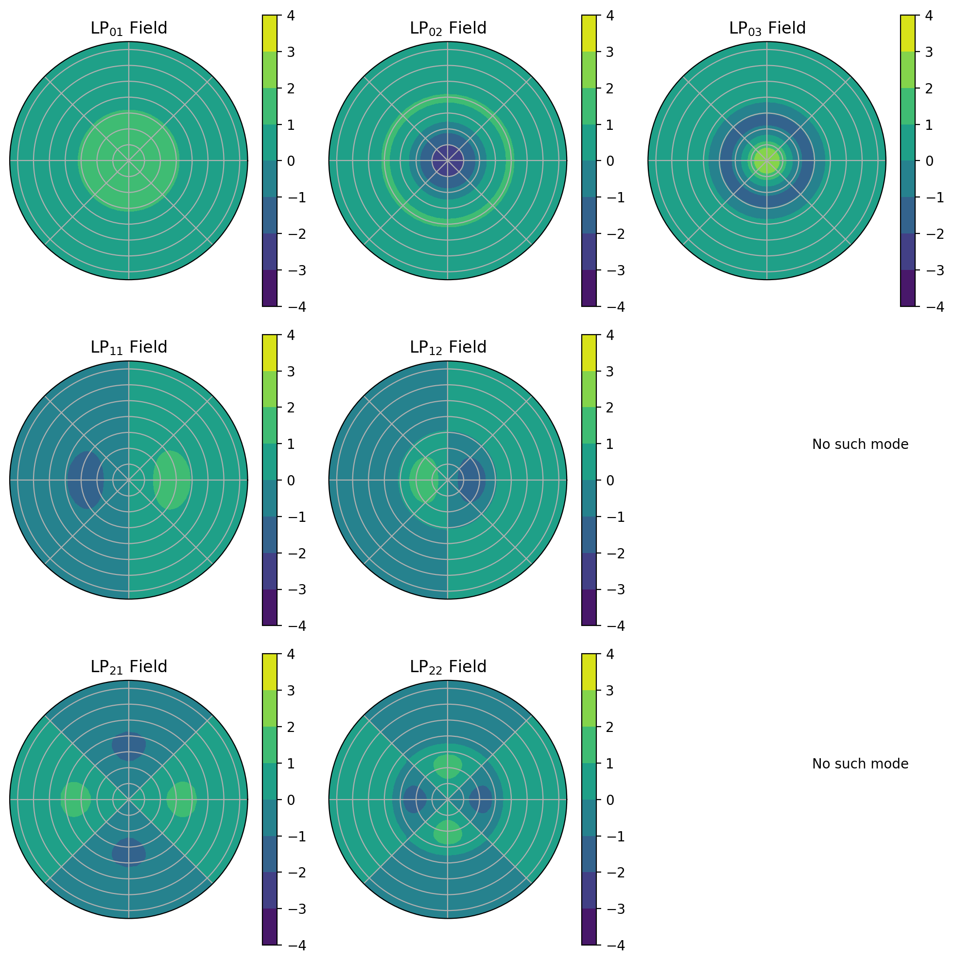
[10]:
V = 8
r_over_a = np.linspace(0, 1.5, 50)
phi = np.linspace(0, 2 * np.pi, 40)
clevs = np.linspace(-4, 4, 9)

fig, axs = plt.subplots(3, 3, figsize=(10, 10), subplot_kw={"polar": True})  # Use subplot_kw to specify polar

axs = axs.flatten()  # Flatten the array to simplify index access

for idx, ax in enumerate(axs):
    ell = idx // 3
    em = idx % 3 + 1

    b = ofiber.LP_mode_value(V, ell, em)
    if b is None:
        ax.axis("off")  # Turn off axis if no mode exists
        ax.annotate(
            "No such mode", xy=(0.5, 0.5), ha="center", va="center", transform=ax.transAxes
        )  # Use transAxes for positioning
        continue

    r_field = ofiber.LP_radial_field(V, b, ell, r_over_a)
    phi_field = np.cos(ell * phi)
    R, PHI = np.meshgrid(r_over_a, phi)
    R_FIELD, PHI_FIELD = np.meshgrid(phi_field, r_field)
    Z = R_FIELD * PHI_FIELD

    cax = ax.contourf(phi, r_over_a, Z, levels=clevs)
    ax.set_xticklabels([])  # Remove x tick labels
    ax.set_yticklabels([])  # Remove y tick labels
    ax.set_title(r"LP$_{%d%d}$ Field" % (ell, em))

    fig.colorbar(cax, ax=ax)

plt.tight_layout()  # Adjust layout
plt.show()
[11]:
V = 8

r_over_a = np.linspace(0, 1.5, 50)
phi = np.linspace(0, 2 * np.pi, 40)
R, PHI = np.meshgrid(r_over_a, phi)

clevs = np.linspace(-4, 4, 9)
dlevs = np.linspace(0, 8, 9)

fig = plt.figure(figsize=(10, 40))  # Adjusted to create only a figure without an unused axis

graph = 0
rows = 8
cols = 2
for ell in range(5):
    phi_field = np.cos(ell * phi)

    for em in [1, 2]:

        b = ofiber.LP_mode_value(V, ell, em)
        if b is None:
            continue
        r_field = ofiber.LP_radial_field(V, b, ell, r_over_a)
        R_FIELD, PHI_FIELD = np.meshgrid(phi_field, r_field)
        Z = R_FIELD * PHI_FIELD

        graph += 1

        ax = plt.subplot(rows, cols, graph, polar=True)
        cax = ax.contourf(phi, r_over_a, Z, levels=clevs)
        ax.set_xticklabels([])
        ax.set_yticklabels([])
        fig.colorbar(cax, ax=ax)
        ax.set_title(r"LP$_{%d%d}$ Field" % (ell, em))

        graph += 1
        Z = Z * Z

        ax = plt.subplot(rows, cols, graph, polar=True)
        cax = ax.contourf(phi, r_over_a, Z, levels=dlevs)
        ax.set_xticklabels([])
        ax.set_yticklabels([])
        fig.colorbar(cax, ax=ax)
        ax.set_title(r"LP$_{%d%d}$ Irradiance" % (ell, em))

plt.show()
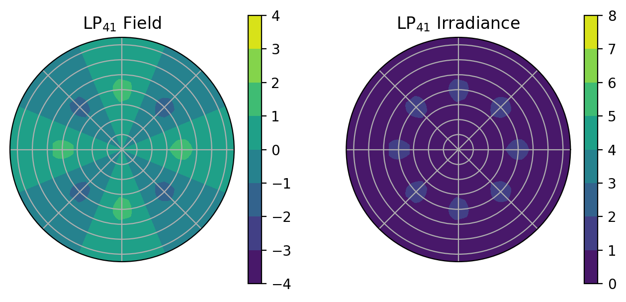
[29]:
V = 8

r_over_a = np.linspace(0, 1.5, 50)
phi = np.linspace(0, 2 * np.pi, 40)
R, PHI = np.meshgrid(r_over_a, phi)

clevs = np.linspace(-4, 4, 9)
dlevs = np.linspace(0, 8, 9)

fig = plt.figure(figsize=(8, 3.5))  # Adjusted to create only a figure without an unused axis

ell = 4
em = 1

phi_field = np.cos(ell * phi)

b = ofiber.LP_mode_value(V, ell, em)
r_field = ofiber.LP_radial_field(V, b, ell, r_over_a)
R_FIELD, PHI_FIELD = np.meshgrid(phi_field, r_field)
Z = R_FIELD * PHI_FIELD

ax = plt.subplot(1, 2, 1, polar=True)
cax = ax.contourf(phi, r_over_a, Z, levels=clevs)
ax.set_xticklabels([])
ax.set_yticklabels([])
fig.colorbar(cax, ax=ax)
ax.set_title(r"LP$_{%d%d}$ Field" % (ell, em))

ax = plt.subplot(1, 2, 2, polar=True)
cax = ax.contourf(phi, r_over_a, Z * Z, levels=dlevs)
ax.set_xticklabels([])
ax.set_yticklabels([])
fig.colorbar(cax, ax=ax)
ax.set_title(r"LP$_{%d%d}$ Irradiance" % (ell, em))

plt.show()
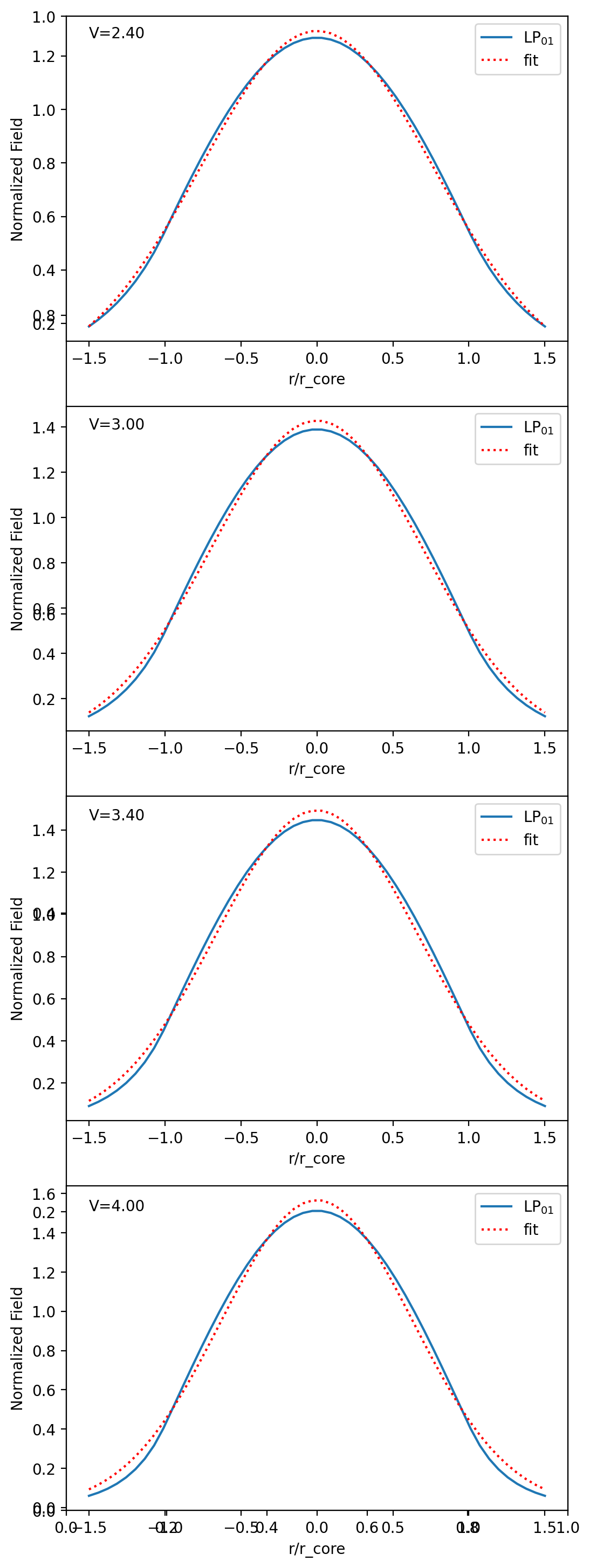
[12]:
def gauss(x, A, w):
    return A * np.exp(-(x**2) / w**2)


r_over_a = np.linspace(-1.5, 1.5, 50)
phi = 0


graph = 1
rows = 4
cols = 1

fig, ax = plt.subplots(figsize=(6, 18))

ell = 0
em = 1

for V in [2.4, 3, 3.4, 4]:

    b = ofiber.LP_mode_value(V, ell, em)
    field = ofiber.LP_radial_field(V, b, ell, r_over_a)

    plt.subplot(rows, cols, graph)
    plt.plot(r_over_a, field, label=r"LP$_{01}$")
    plt.annotate("V=%.2f" % V, xy=(-1.5, max(field)))

    popt, pcov = curve_fit(gauss, r_over_a, field)
    fit = gauss(r_over_a, popt[0], popt[1])
    plt.plot(r_over_a, fit, ":r", label="fit")

    plt.ylabel("Normalized Field")
    plt.xlabel("r/r_core")
    plt.legend()
    graph += 1

plt.show()
Variation of the fractional power contained in the cladding with V
Ghatak Figure 8.11
[13]:
V = np.linspace(0.1, 12, 100)

plt.figure(figsize=(8, 4.5))
ell = 0
for ell in [0, 1, 2]:

    for em in [1, 2]:

        ratio = np.zeros_like(V)
        for i in range(len(V)):
            b = ofiber.LP_mode_value(V[i], ell, em)
            if b is None:
                continue
            clad = ofiber.LP_clad_irradiance(V[i], b, ell)
            total = ofiber.LP_total_irradiance(V[i], b, ell)
            ratio[i] = clad / total

        j = np.nanargmax(ratio)
        plt.annotate("LP%d%d" % (ell, em), xy=(V[j], ratio[j]))

        plt.plot(V, ratio)
plt.xlabel("V-parameter")
plt.ylabel(r"$P_{clad}/P_{total}$")
plt.ylim(0, 1.1)
plt.title("Cladding Fraction in Step-Index Fiber")
plt.show()

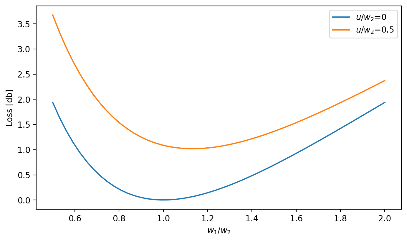
Variation of loss at a perfectly aligned joint between two single-mode fibers
Ghatak Figure 8.14
[14]:
plt.figure(figsize=(8, 4.5))

w1 = np.linspace(0.5, 2, 50)
w2 = np.ones_like(w1)

loss_db = ofiber.transverse_misalignment_loss_db(w1, w2, 0)
plt.plot(w1, loss_db, label=r"$u/w_2$=0")

loss_db = ofiber.transverse_misalignment_loss_db(w1, w2, 0.5)
plt.plot(w1, loss_db, label=r"$u/w_2$=0.5")

plt.xlabel(r"$w_1/w_2$")
plt.ylabel("Loss [db]")
plt.legend()
plt.show()
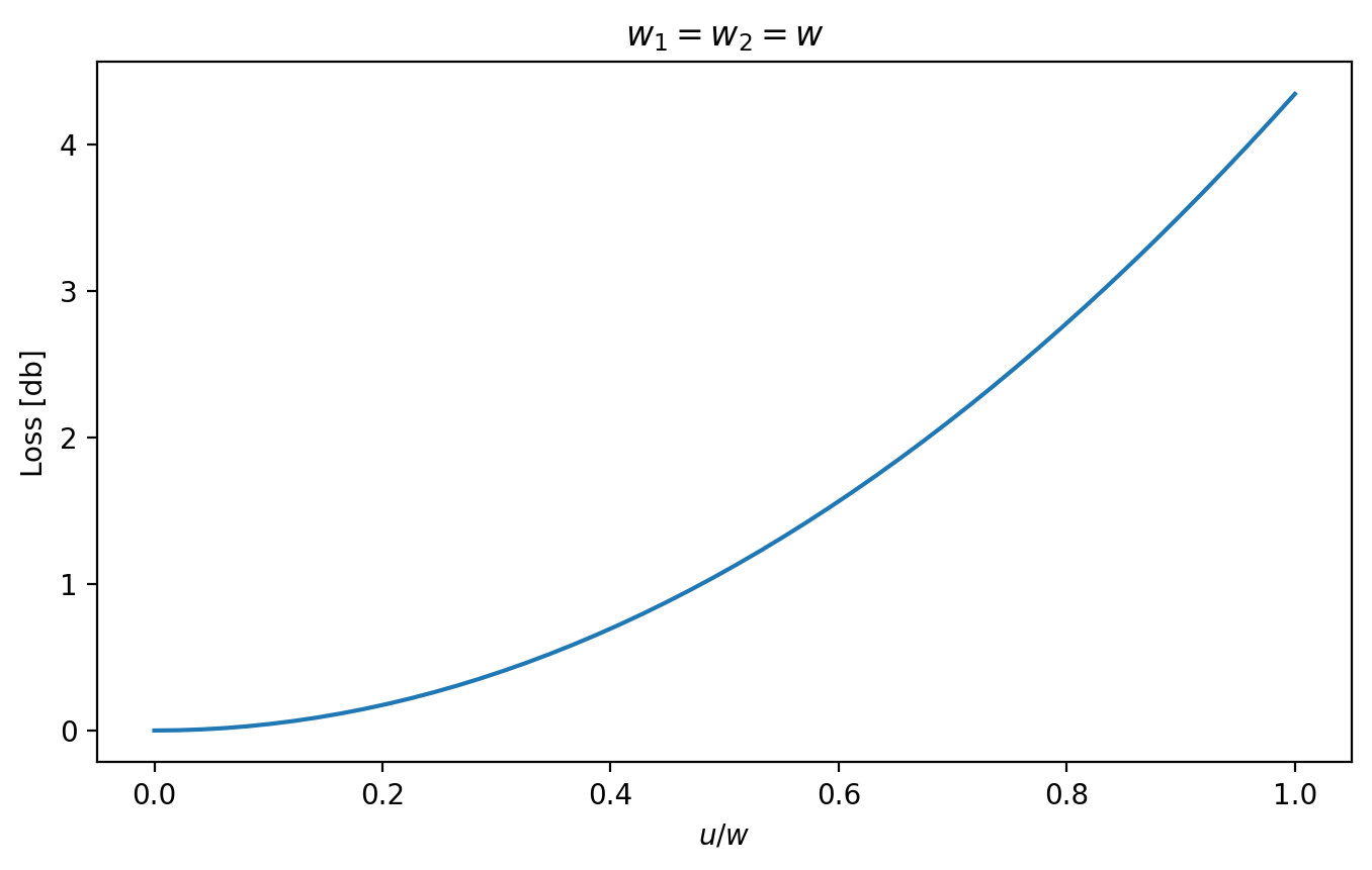
[15]:
u = np.linspace(0, 1, 50)

plt.figure(figsize=(8, 4.5))
loss_db = ofiber.transverse_misalignment_loss_db(1, 1, u)
plt.plot(u, loss_db)

plt.xlabel(r"$u/w$")
plt.ylabel("Loss [db]")
plt.title(r"$w_1=w_2=w$")
plt.show()
[ ]: