Refractive Indices of Glasses

Scott Prahl

Sept 2023

The interface is a bit weird. Basically, you need to get the Sellmeier coefficients for the type of glass that you want. Fortunately, this module has a bunch of glasses entered already. The list is named ALL_GLASS_NAMES.

%config InlineBackend.figure_format='retina'

import sys
import scipy
import numpy as np
import matplotlib.pyplot as plt

if sys.platform == "emscripten":
    import micropip
    await micropip.install("ofiber")

import ofiber

print(ofiber.ALL_GLASS_NAMES)

['SiO2' 'GeO2' '9.1% P2O2' '13.3% B2O3' '1.0% F' '16.9% Na2O : 32.5% B2O3'
 'ABCY' 'HBL' 'ZBG' 'ZBLA' 'ZBLAN' '5.2% B2O3' '10.5% P2O2' 'N-BK7'
 'fused silica' 'sapphire (ordinary)' 'sapphire (extraordinary)'
 'MgF2 (ordinary)' 'MgF2 (extraordinary)' 'CaF2' 'F2' 'F5' 'FK5HTi' 'K10'
 'K7' 'LAFN7' 'LASF35' 'LF5' 'LF5HTi' 'LLF1' 'LLF1HT' 'N-BAF1' 'N-BAF4'
 'N-BAF5' 'N-BAF5' 'N-BAK1' 'N-BAK2' 'N-BAK4' 'N-BALF' 'N-BALF' 'N-BASF'
 'N-BASF' 'N-BK10' 'N-F2' 'N-FK5' 'N-FK51' 'N-FK58' 'N-K5' 'N-KF9'
 'N-KZFS' 'N-KZFS' 'N-KZFS' 'N-KZFS' 'N-KZFS' 'N-LAF2' 'N-LAF2' 'N-LAF3'
 'N-LAF3' 'N-LAF3' 'N-LAF7' 'N-LAK1' 'N-LAK1' 'N-LAK1' 'N-LAK2' 'N-LAK2'
 'N-LAK3' 'N-LAK3' 'N-LAK7' 'N-LAK8' 'N-LAK9' 'N-LASF' 'N-LASF' 'N-LASF'
 'N-LASF' 'N-LASF' 'N-LASF' 'N-LASF' 'N-LASF' 'N-LASF' 'N-PK51' 'N-PK52'
 'N-PSK3' 'N-PSK5' 'N-SF1' 'N-SF10' 'N-SF11' 'N-SF14' 'N-SF15' 'N-SF2'
 'N-SF4' 'N-SF5' 'N-SF57' 'N-SF6' 'N-SF66' 'N-SF6H' 'N-SF8' 'N-SK11'
 'N-SK14' 'N-SK16' 'N-SK2' 'N-SK4' 'N-SK5' 'N-SSK2' 'N-SSK5' 'N-SSK8'
 'N-ZK7' 'N-ZK7A' 'P-BK7' 'P-LAF3' 'P-LAK3' 'P-LASF' 'P-LASF' 'P-LASF'
 'P-SF68' 'P-SF69' 'P-SF8' 'P-SK57' 'P-SK57' 'P-SK58' 'P-SK60' 'SF1'
 'SF10' 'SF11' 'SF2' 'SF4' 'SF5' 'SF56A' 'SF57']

You can just count to find the glass you want. Standard silicon dioxide SiO₂ has number 0. Germanium dioxide GeO₂ has number 1.

Alternatively you can search for the glass you want. The number of BK7 is 13.

ofiber.find_glass("BK7")

13

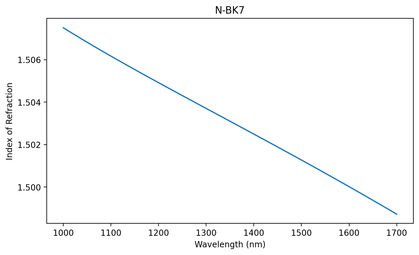
So ofiber.glass(13) will return the coefficients for BK7 glass for example. The function ofiber.n(glass,λ) returns the index of refraction at a particular (vacuum) wavelength \(\lambda_0\).

glass_coefficients = ofiber.glass(13)
name = ofiber.glass_name(13)
λ = np.linspace(1000, 1700, 100) * 1e-9
n = ofiber.n(glass_coefficients, λ)
plt.figure(figsize=(8, 4.5))
plt.plot(λ * 1e9, n)
plt.title(name)
plt.xlabel("Wavelength (nm)")
plt.ylabel("Index of Refraction")
plt.show()

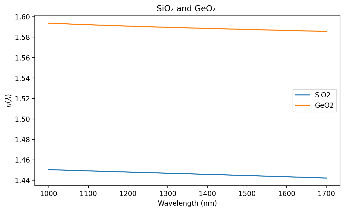
SiO₂ and GeO₂ fibers

These are the mainstay of the optical fiber industry. By doping SiO₂ with GeO₂ different refractive index profiles can be achieved. This plot shows the limits of 100% of each material. They look pretty similar, just displaced by 0.14 index units.

glass = ofiber.glass(0)
name = ofiber.glass_name(0)
λ = np.linspace(1000, 1700, 100) * 1e-9
n = ofiber.n(glass, λ)
plt.figure(figsize=(8, 4.5))
plt.plot(λ * 1e9, n, label=name)

glass = ofiber.glass(1)
name = ofiber.glass_name(1)
λ = np.linspace(1000, 1700, 100) * 1e-9
n = ofiber.n(glass, λ)
plt.plot(λ * 1e9, n, label=name)

plt.title("SiO₂ and GeO₂ ")
plt.xlabel("Wavelength (nm)")
plt.ylabel(r"$n(\lambda)$")
plt.legend()
plt.show()

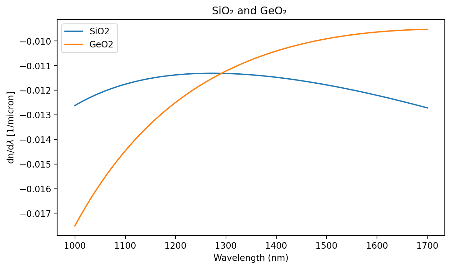
However, if you plot the first derivative, interesting things appear. Notice the weird units on the vertical axis.

glass = ofiber.glass(0)
name = ofiber.glass_name(0)
λ = np.linspace(1000, 1700, 100) * 1e-9
dn = ofiber.dn(glass, λ)
plt.figure(figsize=(8, 4.5))
plt.plot(λ * 1e9, dn * 1e-6, label=name)

glass = ofiber.glass(1)
name = ofiber.glass_name(1)
λ = np.linspace(1000, 1700, 100) * 1e-9
dn = ofiber.dn(glass, λ)
plt.plot(λ * 1e9, dn * 1e-6, label=name)

plt.title("SiO₂ and GeO₂ ")
plt.xlabel("Wavelength (nm)")
plt.ylabel(r"dn/d$\lambda$ [1/micron]")
plt.legend()
plt.show()

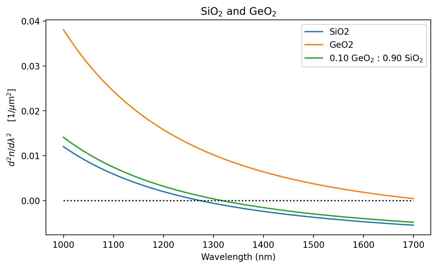
SiO₂ doped with GeO₂

Since doping of SiO₂ with GeO₂ is common there is a special routine to generate Sellmeier coefficients for glass doped with a specific fraction \(x\) of GeO₂. The interface is simple.

help(ofiber.doped_glass)

Help on function doped_glass in module ofiber.refraction:

doped_glass(x)
    Calculate Sellmeier coefficients for SiO_2 doped with GeO_2.

    The idea is that the glass a combination of silicon dioxide or
    germanium dioxide where x is the molar fraction of GeO_2. Thus
    (1-x) is the molar fraction of SiO_2.  The overall composition is
    x * GeO_2 : (1 - x) * SiO_2.

    Args:
        x: fraction of GeO_2 (0<=x<=1)

    Returns:
        Sellmeier coefficients for doped glass (array of six values)

Here the second derivative of the refractive index is plotted for 100% SiO₂, 100% GeO₂, and 10% GeO₂

glass = ofiber.glass(0)
name = ofiber.glass_name(0)
λ = np.linspace(1000, 1700, 100) * 1e-9
d2n = ofiber.d2n(glass, λ)
plt.figure(figsize=(8, 4.5))
plt.plot(λ * 1e9, d2n * 1e-12, label=name)

glass = ofiber.glass(1)
name = ofiber.glass_name(1)
λ = np.linspace(1000, 1700, 100) * 1e-9
d2n = ofiber.d2n(glass, λ)
plt.plot(λ * 1e9, d2n * 1e-12, label=name)

glass = ofiber.doped_glass(0.10)
name = ofiber.doped_glass_name(0.1)
λ = np.linspace(1000, 1700, 100) * 1e-9
d2n = ofiber.d2n(glass, λ)
plt.plot(λ * 1e9, d2n * 1e-12, label=name)

plt.plot([1000, 1700], [0, 0], ":k")
plt.title("SiO$_2$ and GeO$_2$")
plt.xlabel("Wavelength (nm)")
plt.ylabel(r"$d^2n/d\lambda^2$    [1/$\mu$m$^2$]")
plt.legend()
plt.show()

If we just want the second derivative at a specific wavelength, that is simple too. The only tricky part is converting from the default 1/m\(^2\) to 1/µm\(^2\)

λ = 1550e-9
glass = ofiber.glass(0)
name = ofiber.glass_name(0)
disp = ofiber.d2n(glass, λ)
print("d^2n/dlambda^2 of %s at %.0f nm is %.4f/um**2" % (name, λ * 1e9, disp * 1e-12))

d^2n/dlambda^2 of SiO2 at 1550 nm is -0.0042/um**2

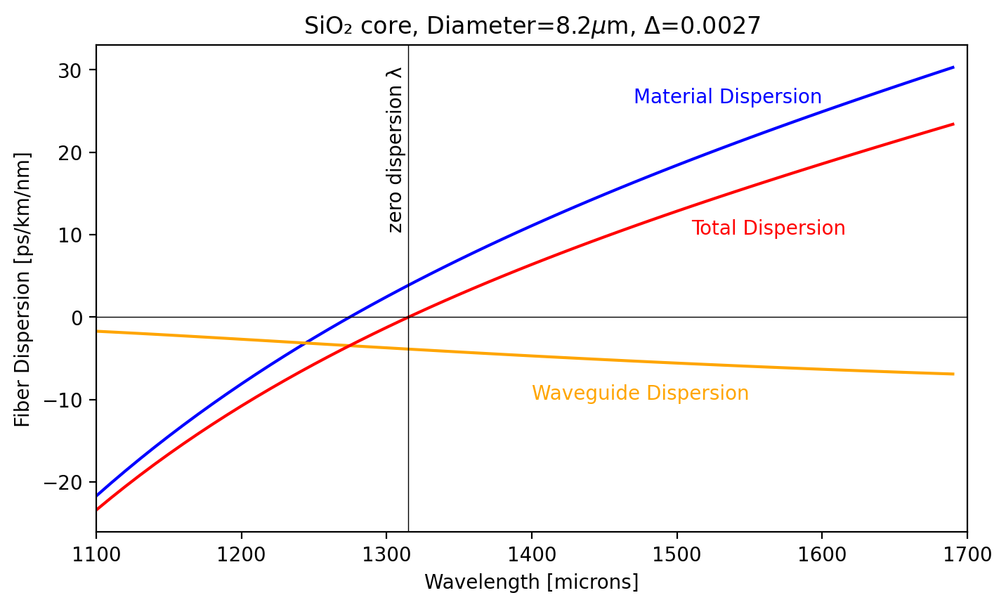
We use this to calculate the material, waveguide, and total dispersion for a fiber. (These are available directly in the ofiber.dispersion module. This is just an example.)

# Ghatak Section 3.A.1, page 85.
#
c = 3e8  # [m/s]

a = 4.1e-6  # [m] Fiber radius
delta = 0.0027  # Fractional change in the index of refraction

start = 1100
finish = 1700
resolution = 10

λ = np.arange(start, finish, resolution) * 1e-9
npoints = len(λ)

glass = ofiber.doped_glass(0)
n1 = ofiber.n(glass, λ)
d2n = ofiber.d2n(glass, λ)

V = (2 * np.pi / λ) * a * n1 * np.sqrt(2 * delta)

# Material Dispersion
M = -(λ / c) * d2n

# Waveguide dispersion
Dw = -n1 * (1 + delta) * delta / c / λ * (0.080 + 0.549 * (2.834 - V) ** 2)

ps_nm_km = 1e-12 / 1e-9 / 1e3
plt.subplots(1, 1, figsize=(8, 4.5))
plt.plot(λ * 1e9, M / ps_nm_km, color="blue")

plt.plot(λ * 1e9, Dw / ps_nm_km, color="orange")
plt.plot(λ * 1e9, (M + Dw) / ps_nm_km, color="red")
plt.axhline(0, color="black", linewidth=0.5)
plt.xlabel("Wavelength [microns]")
plt.ylabel("Fiber Dispersion [ps/km/nm]")
plt.title(r"SiO₂ core, Diameter=%.1f$\mu$m, Δ=%.4f" % (a * 2e6, delta))
plt.xlim(1100, 1700)
plt.text(1510, 10, "Total Dispersion", color="red")
plt.text(1600, 26, "Material Dispersion", color="blue", ha="right")
plt.text(1400, -10, "Waveguide Dispersion", color="orange")
plt.axvline(1315, color="black", linewidth=0.5)
plt.text(1300, 10, " zero dispersion λ", rotation=90)
# plt.savefig('dispersion.svg')
plt.show()