Symmetric Planar Waveguides

Scott Prahl

Sept 2023

Planar waveguides are a strange abstraction. These are waveguides that are sandwiches with a specified thickness but are infinite in extent in the other directions. Studying planar waveguides before cylindrical waveguides is done because the math is simpler (solutions are trignometric functions instead of Bessel functions) and therefore it is a bit less likely that one will get lost in the math.

%config InlineBackend.figure_format='retina'

import sys
import scipy
import numpy as np
import matplotlib.pyplot as plt

if sys.platform == "emscripten":
    import micropip
    await micropip.install("ofiber")

import ofiber

Modes in planar waveguides

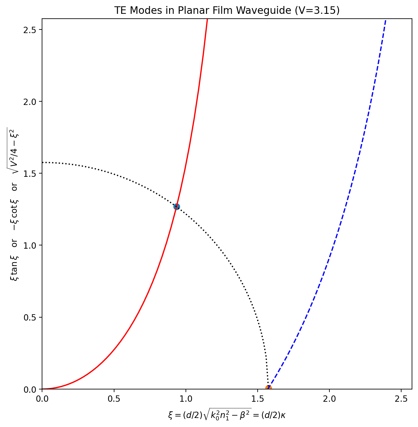
V=3.15

V = 3.15
xx = ofiber.TE_crossings(V)
aplt = ofiber.TE_mode_plot(V)
yy = np.sqrt((V / 2) ** 2 - xx[0::2] ** 2)
aplt.scatter(xx[0::2], yy, s=50)
yy = np.sqrt((V / 2) ** 2 - xx[1::2] ** 2)
aplt.scatter(xx[1::2], yy, s=50)

aplt.show()

V=4.77

n1 = 1.503
n2 = 1.5
lambda0 = 0.5e-6
k = 2 * np.pi / lambda0
NA = np.sqrt(n1**2 - n2**2)
d = 4e-6

V = k * d * NA
xx = ofiber.TE_crossings(V)

b = 1 - (2 * xx / V) ** 2
beta = np.sqrt((n1**2 - n2**2) * b + n2**2)
theta = np.arccos(beta / n1) * 180 / np.pi

aplt = ofiber.TE_mode_plot(V)
yy = np.sqrt((V / 2) ** 2 - xx[0::2] ** 2)
aplt.scatter(xx[0::2], yy, s=50)
yy = np.sqrt((V / 2) ** 2 - xx[1::2] ** 2)
aplt.scatter(xx[1::2], yy, s=50)
aplt.show()

print(xx)
print("b       =", b)
print("beta hat=", beta)
print("theta   =", theta, " degrees")

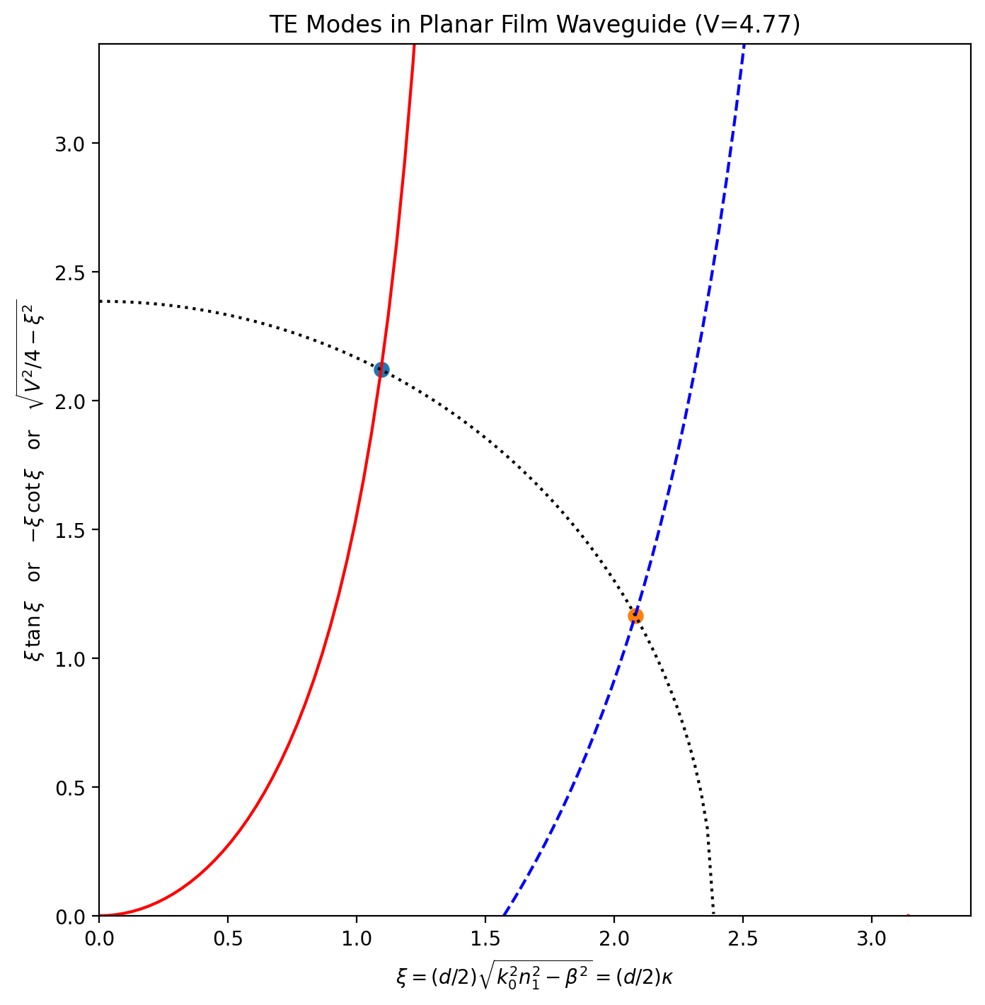
[1.09425217 2.08131807]
b       = [0.78958411 0.23876175]
beta hat= [1.50236925 1.50071683]
theta   = [1.6599766  3.15850983]  degrees

V=5.5

V = 5.5
xx = ofiber.TE_crossings(V)
aplt = ofiber.TE_mode_plot(V)
yy = np.sqrt((V / 2) ** 2 - xx[0::2] ** 2)
aplt.scatter(xx[0::2], yy, s=50)
yy = np.sqrt((V / 2) ** 2 - xx[1::2] ** 2)
aplt.scatter(xx[1::2], yy, s=50)

aplt.show()

print("cutoff wavelength = %.0f nm" % (2 * d * NA * 1e9))

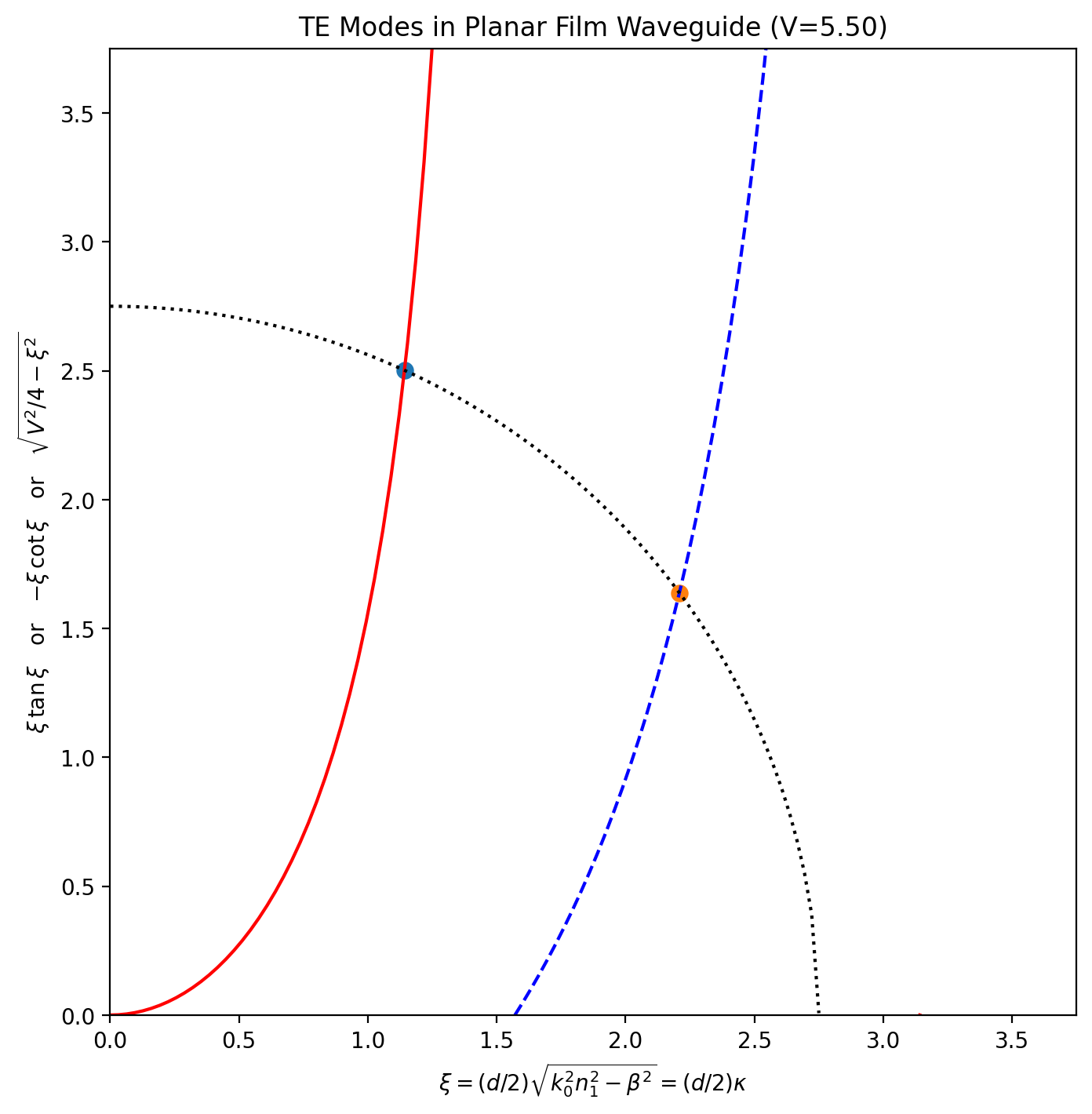
cutoff wavelength = 759 nm

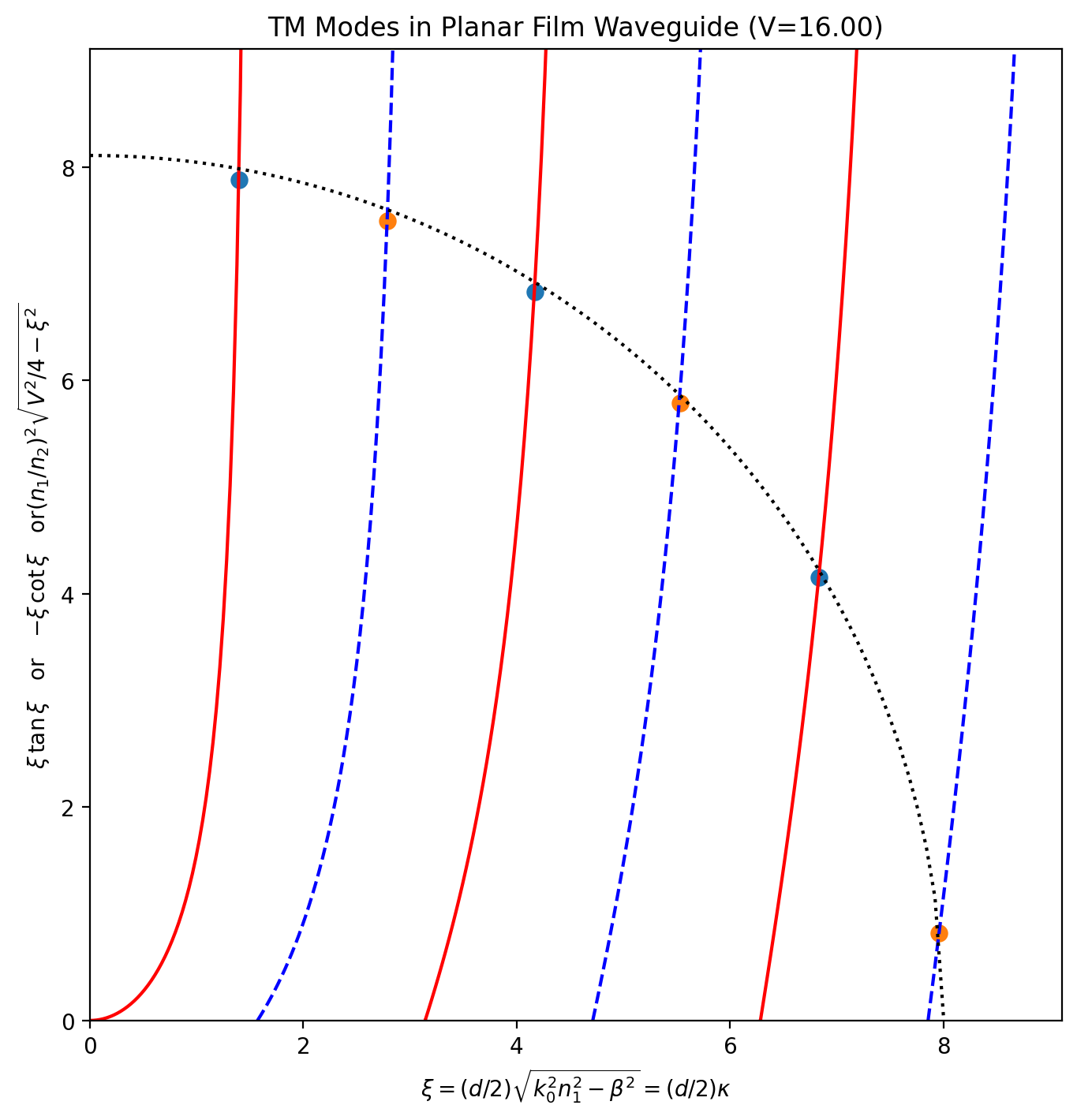
V=16

V = 16
n1 = 1.5
n2 = 1.49
xx = ofiber.TM_crossings(V, n1, n2)

aplt = ofiber.TM_mode_plot(V, n1, n2)
yy = np.sqrt((V / 2) ** 2 - xx[0::2] ** 2)
aplt.scatter(xx[0::2], yy, s=50)
yy = np.sqrt((V / 2) ** 2 - xx[1::2] ** 2)
aplt.scatter(xx[1::2], yy, s=50)

aplt.show()

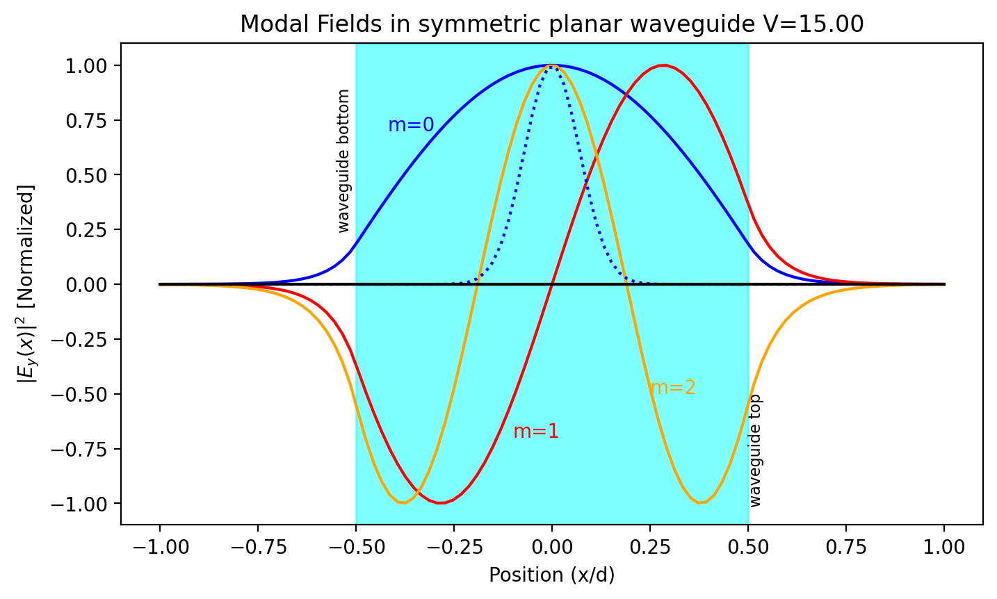
Internal field inside waveguide

V = 15
d = 1
x = np.linspace(-1, 1, 100)

plt.figure(figsize=(8, 4.5))
m = 0
plt.plot(x, ofiber.TE_field(V, d, x, m), color="blue")
plt.text(-0.42, 0.7, "m=%d" % m, color="blue")

m = 1
plt.plot(x, ofiber.TE_field(V, d, x, m), color="red")
plt.text(-0.10, -0.7, "m=%d" % m, color="red")

m = 2
plt.plot(x, ofiber.TE_field(V, d, x, m), color="orange")
plt.text(0.25, -0.5, "m=%d" % m, color="orange")

plt.plot(x, np.exp(-(x**2) / 0.01), ":b")
plt.plot([-1, 1], [0, 0], "k")

plt.axvspan(-0.5, 0.5, color="cyan", alpha=0.5)
plt.text(-0.55, 0.25, "waveguide bottom", rotation=90, fontsize=8)
plt.text(0.5, -1, "waveguide top", rotation=90, fontsize=8)

plt.xlabel("Position (x/d)")
plt.ylabel("$|E_y(x)|^2$ [Normalized]")
plt.title("Modal Fields in symmetric planar waveguide V=%.2f" % V)
# plt.savefig('planarwaveguide.svg')
plt.show()

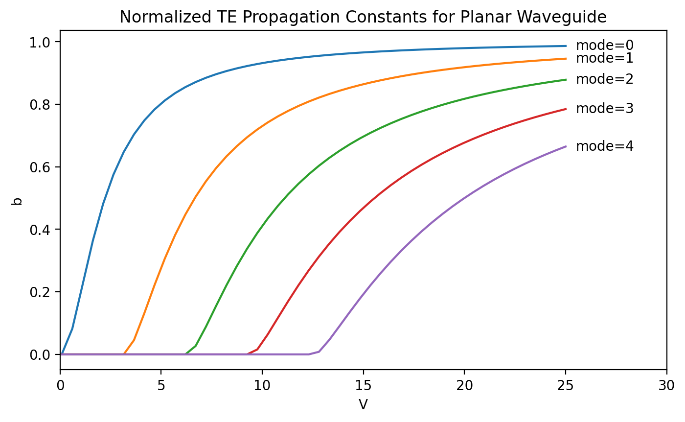
TE propagation constants for first five modes

plt.figure(figsize=(8, 4.5))

V = np.linspace(0.1, 25, 50)
for mode in range(5):
    b = ofiber.TE_propagation_constant(V, mode)
    plt.plot(V, b)
    plt.text(25.5, b[-1], "mode=%d" % mode, va="center")

plt.xlabel("V")
plt.ylabel("b")
plt.title("Normalized TE Propagation Constants for Planar Waveguide")
plt.xlim(0, 30)
plt.show()

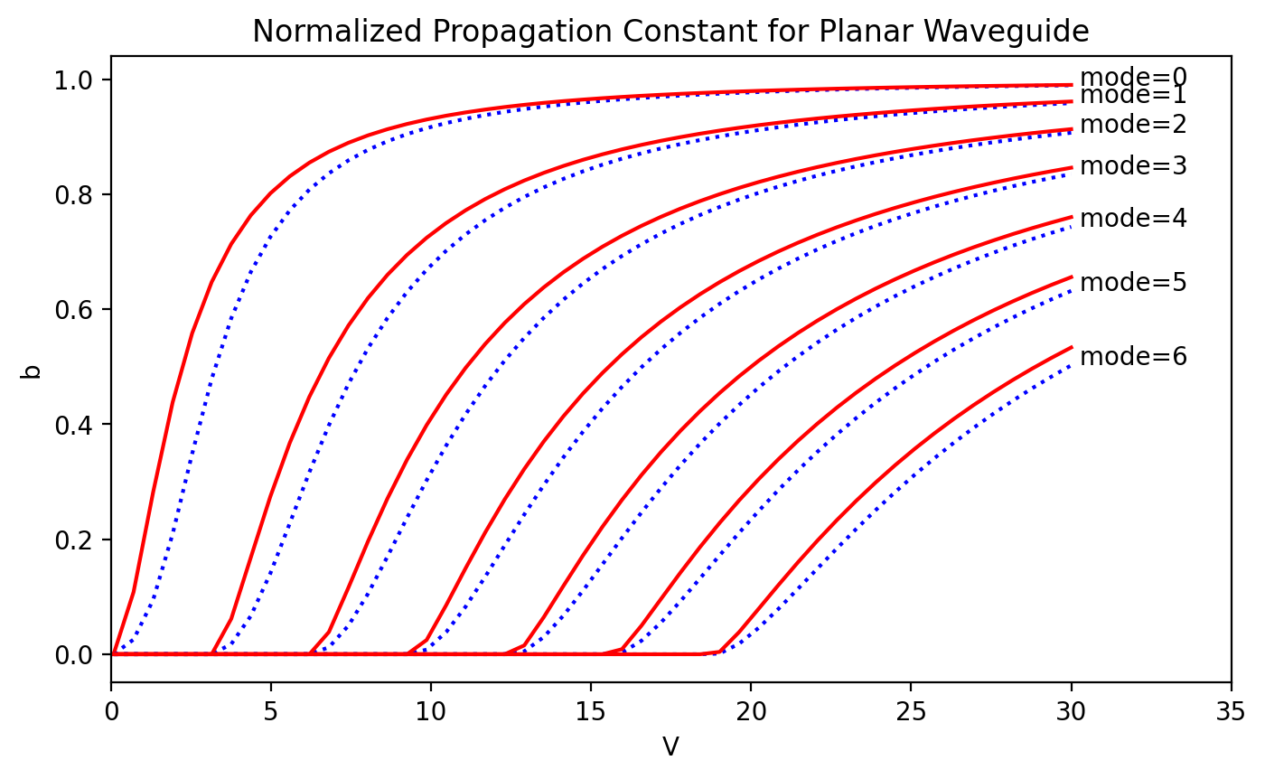
TE & TM propagation constants for first five modes

plt.figure(figsize=(8, 4.5))
n1 = 1.5
n2 = 1.0
V = np.linspace(0.1, 30, 50)
for mode in range(7):
    b = ofiber.TM_propagation_constant(V, n1, n2, mode)
    plt.annotate(" mode=%d" % mode, xy=(30, b[-1]))
    plt.plot(V, b, ":b")
    b = ofiber.TE_propagation_constant(V, mode)
    plt.plot(V, b, "r")

plt.xlabel("V")
plt.ylabel("b")
plt.title("Normalized Propagation Constant for Planar Waveguide")
plt.xlim(0, 35)
plt.show()